Code
data("calcium", package = "SMPracticals")
plot(cal ~ time, data = calcium,
     xlab = "Time (minutes)",
     ylab = "Calcium uptake (nmoles/mg)",
     bg = "#ff7518", pch = 21)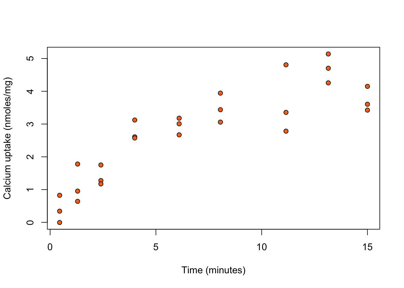
The combination of some data and an aching desire for an answer does not ensure that a reasonable answer can be extracted from a given body of data.
— John W. Tukey (1915–2000)
in Tukey (1986). Sunset Salvo. The American Statistician, 40 (1), p. 74.
So far we have only considered models where the link function of the mean response is equal to a linear predictor. For example, GLMMs, which are the most general models we have seen so far, have \[ \begin{aligned} Y_i \mid x_i, z_i, b & \stackrel{\text{ind}}{\sim}\mathop{\mathrm{EF}}(\mu_i,\sigma^2)\,,\\ \begin{bmatrix} g(\mu_1)\\\vdots \\ g(\mu_n) \end{bmatrix} & = \eta = X \beta + Zb \, ,\\ b & \sim {\mathop{\mathrm{N}}}(0,\Sigma_b)\,, \end{aligned} \tag{3.1}\] where \(\mathop{\mathrm{EF}}(\mu_i,\sigma^2)\) is an exponential family distribution with mean \(\mu_i\) and variance \(\sigma^2 V(\mu_i) / m_i\) for known \(m_i\). The key point is that the predictor \(\eta\) is a linear function of the parameters. Linear models, generalized linear models and linear mixed models are all special cases of the GLMM.
Models with linear predictors form the basis of most applied statistical analyses. It is often the case, though, that there is no scientific reason to believe these linear models are true for a given application.
We begin by considering nonlinear extensions of the normal linear model \[ Y_i = x_i^\top \beta + \epsilon_i \,, \tag{3.2}\] where \(\epsilon_1, \ldots, \epsilon_n\) are independent with \(\epsilon_i \sim {\mathop{\mathrm{N}}}(0, \sigma^2)\), and \(\beta\) are the \(p\) regression parameters.
Instead of the mean response being the linear predictor \(x_i^\top \beta\), we may allow it to be a nonlinear function of parameters, that is \[ Y_i = \eta(x_i, \beta) + \epsilon_i \,, \tag{3.3}\] where \(\epsilon_1, \ldots, \epsilon_n\) are independent with \(\epsilon_i \sim {\mathop{\mathrm{N}}}(0, \sigma^2)\), and \(\eta(x_i, \beta)\) is a nonlinear function of covariates and parameters \(\beta\).
The linear model (3.2) is a special case of the model specified by (3.3) for \(\eta(x, \beta) = x^\top \beta\).
Parameters in nonlinear models can be of two different types:
Physical parameters that have particular meaning in the subject-area where the model comes from. Estimating the value of physical parameters, then, contributes to scientific understanding.
Tuning parameters that do not necessarily have any physical meaning. Their presence is justified as a simplification of a more complex underlying system. The aim when estimating them is to make the model represent reality as well as possible.
The function \(\eta(x, \beta)\) can be specified in two ways:
Mechanistically: prior scientific knowledge is incorporated into building a mathematical model for the mean response. That model can often be complex and \(\eta(x, \beta)\) may not be available in closed form.
Phenomenologically (empirically): a function \(\eta(x, \beta)\) may be posited that appears to capture the non-linear nature of the mean response.
Example 3.1 (Calcium uptake) The calcium dataset in the SMPracticals R package provides data on the uptake of calcium (cal; in nmoles per mg) at set times (time; in minutes) by \(27\) cells in “hot” suspension. Figure 3.1 shows calcium uptake against time.
data("calcium", package = "SMPracticals")
plot(cal ~ time, data = calcium,
xlab = "Time (minutes)",
ylab = "Calcium uptake (nmoles/mg)",
bg = "#ff7518", pch = 21)We see that calcium uptake grows with time. There is a large class of phenomenological models for growth curves.
Consider the non-linear model with \[ \eta(x, \beta) = \beta_0 \left( 1 - \exp \left( - x / \beta_1 \right) \right) \, . \tag{3.4}\] This is derived by assuming that the rate of growth is proportional to the calcium remaining, i.e. \[ \frac{d \eta}{d x} = (\beta_0 - \eta)/\beta_1 \, . \] The solution to this differential equation, with initial condition \(\eta(0,\beta) = 0\), is (3.4). Here, \(\beta_0\) is the calcium uptake after infinite time, and \(\beta_1\) controls its growth rate.
We use R to fit a model assumes a linear relationship of calcium uptake with time, a model that assumes a quadratic relationship, and the model specified by (3.4).
calc_lm1 <- lm(cal ~ time, data = calcium)
calc_lm2 <- lm(cal ~ time + I(time^2), data = calcium)
calc_nlm <- nls(cal~ beta0 * ( 1 - exp(-time/beta1)), data = calcium,
                start = list(beta0 = 5, beta1 = 5))
Figure 3.2 shows fitted curves for the three different models overlaid on the scatterplot of calcium uptake against time.
newdata <- data.frame(time = seq(min(calcium$time), max(calcium$time), length.out = 100))
pred_lm1 <- predict(calc_lm1, newdata = newdata)
pred_lm2 <- predict(calc_lm2, newdata = newdata)
pred_nlm <- predict(calc_nlm, newdata = newdata)
plot(cal ~ time, data = calcium,
     xlab = "Time (minutes)",
     ylab = "Calcium uptake (nmoles/mg)",
     bg = "#ff7518", pch = 21)
lines(newdata$time, pred_lm1, col = gray(0.8), lty = 1, lwd = 2)
lines(newdata$time, pred_lm2, col = gray(0.6), lty = 2, lwd = 2)
lines(newdata$time, pred_nlm, col = gray(0.4), lty = 3, lwd = 2)
legend("bottomright", legend = c("LM (linear)", "LM (quadratic)", "NLM"),
       col = gray(c(0.8, 0.6, 0.4)), lty = 1:3, lwd = 2)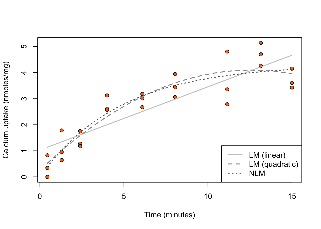
A comparison of the three models in terms of number of parameters, maximized log-likelihood value, and AIC and BIC returns
models <- list(`LM (linear)` = calc_lm1,
               `LM (quadratic)` = calc_lm2,
               `NLM` = calc_nlm)
out <- sapply(models, function(m) {
    c(p = length(coef(m)),
      loglik = logLik(m),
      AIC = AIC(m),
      BIC = BIC(m))
})
round(t(out), 3)
p loglik AIC BIC
LM (linear) 2 -28.701 63.403 67.290
LM (quadratic) 3 -20.955 49.910 55.093
NLM 2 -20.955 47.909 51.797The maximized log-likelihoods from the quadratic and nonlinear model are identical up to 3 decimal places. The nonlinear model has is more parsimonious with fewer parameters. As a result it has lower AIC and BIC, and would be the preferred model.
Example 3.2 (Theophylline data) Theophylline is an anti-asthmatic drug. An experiment was performed on \(12\) individuals to investigate the way in which the drug leaves the body. The study of drug concentrations inside organisms is called pharmacokinetics.
An oral dose was given to each individual at time \(t = 0\), and the concentration of theophylline in the blood was then measured at 11 time points in the next 25 hours.
Let \(Y_{ij}\) be the theophylline concentration (mg/L) for individual \(i\) at time \(t_{ij}\), and \(D_i\) the dose that was administered.
Figure 3.3 shows the concentration of theophylline against time for each of the individuals. There is a sharp increase in concentration followed by a steady decrease.
data("Theoph", package = "datasets")
plot(conc ~ Time, data = Theoph, type = "n",
     ylab = "Concentration (mg/L)", xlab = "Time (hours)")
for (i in 1:30) {
    dat_i <- subset(Theoph, Subject == i)
    lines(conc ~ Time, data = dat_i, col = "grey")
}
points(conc ~ Time, data = Theoph,
       bg = "#ff7518", pch = 21, col = "grey")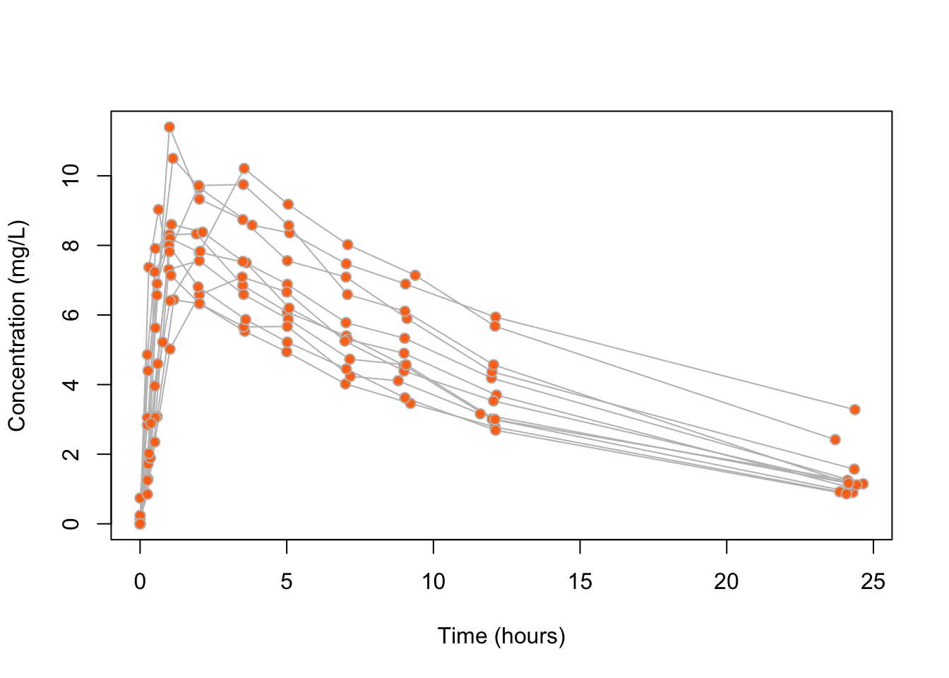
Compartmental models are a common class of model used in pharmacokinetics studies. If the initial dosage is \(D\), then a pharmacokinetic model with a first-order compartment function is \[ \eta(\beta, D,t) = \frac{D \beta_1 \beta_2}{\beta_3(\beta_2 - \beta_1)} \left( \exp \left( - \beta_1 t\right) - \exp \left( - \beta_2 t\right)\right)\,, \tag{3.5}\] where the parameters \(\beta_1, \beta_2, \beta_3\) are all positive and have natural interpretations as follows:
\(\beta_1\): the elimination rate which controls the rate at which the drug leaves the organism;
\(\beta_2\): the absorption rate which controls the rate at which the drug enters the blood;
\(\beta_3\): the clearance which controls the volume of blood for which a drug is completely removed per time unit.
Since all the parameters are positive, and their estimation will most probably require a gradient descent step (e.g. what some of the methods in optim do), it is best to rewrite expression (3.5) in terms of \(\gamma_i = log(\beta_i)\), which can take values on the whole real line. We can write \[
\eta'(\gamma, D, t) = \eta(\beta, D, t) = D \frac{\exp(-\exp(\gamma_1) t) - \exp(-\exp(\gamma_2) t)}{\exp(\gamma_3 - \gamma_1) - \exp(\gamma_3 - \gamma_2)}
\,.
\tag{3.6}\]
Let’s initially ignore the dependence induced from repeated measurements on individuals and fit the nonlinear model \[ Y_{ij} = \eta'(\gamma, D_i,t_{ij}) + \epsilon_{ij} \, , \tag{3.7}\] where \(\epsilon_{ij} \stackrel{\text{ind}}{\sim}{\mathop{\mathrm{N}}}(0,\sigma^2)\).
fm <- conc ~ Dose *
    (exp(-exp(gamma1) * Time) - exp(-exp(gamma2) * Time)) /
    (exp(gamma3 - gamma1) - exp(gamma3 - gamma2))
(pkm <- nls(fm, start = list(gamma1 = 0, gamma2 = -1, gamma3 = -1),
            data = Theoph))
Nonlinear regression model
model: conc ~ Dose * (exp(-exp(gamma1) * Time) - exp(-exp(gamma2) * Time))/(exp(gamma3 - gamma1) - exp(gamma3 - gamma2))
data: Theoph
gamma1 gamma2 gamma3
0.3992 -2.5242 -3.2483
residual sum-of-squares: 274.4
Number of iterations to convergence: 8
Achieved convergence tolerance: 3.709e-06The estimates for \(\beta_1\), \(\beta_2\) and \(\beta_3\) are
setNames(exp(coef(pkm)), paste0("beta", 1:3)) beta1 beta2 beta3
1.49066465 0.08011951 0.03884169 and, using the delta method, the corresponding estimated standard errors are
setNames(exp(coef(pkm)) * coef(summary(pkm))[, "Std. Error"], paste0("beta", 1:3)) beta1 beta2 beta3
0.175208160 0.008840925 0.002889612 Figure 3.4 shows boxplots of the residuals from fitting the model in (3.7), separately for each subject. We see evidence of unexplained differences between individuals.
res <- residuals(pkm, type = "pearson")
ord <- order(ave(res, Theoph$Subject))
subj <- Theoph$Subject[ord]
subj <- factor(subj, levels = unique(subj), ordered = TRUE)
plot(res[ord] ~ subj,
     xlab = "Subject (ordered by mean residual)",
     ylab = "Pearson residual",
     col = "#ff7518", pch = 21)
abline(h = 0, lty = 2)![Residuals for each individual in the theopylline study from model ([-@eq-pkm]).](nonlinear_files/figure-html/fig-theo-resid-1.png)
Further evidence of unexplained differences is found in Figure 3.5, which shows the estimated curves from model (3.7) per individual. Accounting for heterogeneity between individuals seems worthwhile towards getting a better fit.
library("ggplot2")
st <- unique(Theoph[c("Subject", "Dose")])
pred_df <- as.list(rep(NA, nrow(st)))
for (i in seq.int(nrow(st))) {
    pred_df[[i]] <- data.frame(Time = seq(0, 25, by = 0.2),
                               Dose = st$Dose[i],
                               Subject = st$Subject[i])
}
pred_df <- do.call("rbind", pred_df)
pred_df$conc <- predict(pkm, newdata = pred_df)
## Order according to mean residual
theoph <- within(Theoph, Subject <- factor(Subject, levels = unique(subj), ordered = TRUE))
fig_theoph <- ggplot(theoph) +
    geom_point(aes(Time, conc), col = "#ff7518") +
    geom_hline(aes(yintercept = Dose), col = "grey", lty = 3) +
    facet_wrap(~ Subject, ncol = 3) +
    labs(y = "Concentration (mg/L)", x = "Time (hours)") +
    theme_bw()
fig_theoph +
geom_line(data = pred_df, aes(Time, conc), col = "grey") ![Estimated concentrations (grey) for each individual in the theopylline study from model ([-@eq-pkm]). The dotted line is the administered dose.](nonlinear_files/figure-html/fig-theo-fit-1.png)
A nonlinear mixed effects model that accounts for heterogeneity between clusters is \[ Y_{ij} = \eta(\beta + b_i, x_{ij}) + \epsilon_{ij}, \] where \(\epsilon_{ij} \stackrel{\text{ind}}{\sim}{\mathop{\mathrm{N}}}(0,\sigma^2)\), \(b_i \stackrel{\text{ind}}{\sim} {\mathop{\mathrm{N}}}(0,\Sigma_b)\), and \(\Sigma_b\) is a \(q \times q\) covariance matrix.
The above model specifies that \(\beta + b_i\) are parameters specific to the \(i\)th cluster with their relationship to the covariates being perhaps nonlinear.
For example, a mixed effects extension of model (3.7) for the Theophylline data, allows each individual to have distinct log-elimination rate, log-absorption rate and log-clearance, with joint distribution \({\mathop{\mathrm{N}}}(\gamma, \Sigma_b)\). The means \(\gamma\) of the cluster-specific parameters across all individuals are the population parameters. Note that adding normally distributed random variables to \(\gamma_1, \gamma_2, \gamma_3\) (the logarithms of elimination rate, absorption rate and clearance) is less controversial than adding normally distributed random variables to \(\beta_1, \beta_2, \beta_3\), which should be necessarily positive.
It is sometimes useful to specify the model in a way such that only a subset of the parameters can be different for each cluster, and the remainder fixed for all clusters. Suppose there are \(q \le p\) parameters that can be different for each cluster. Then, a more general way of writing the nonlinear mixed model is \[ Y_{ij} = \eta(\beta + A b_i, x_{ij}) + \epsilon_{ij} \,, \tag{3.8}\] where \(\epsilon_{ij} \stackrel{\text{ind}}{\sim}{\mathop{\mathrm{N}}}(0,\sigma^2)\) and \(b_i \stackrel{\text{ind}}{\sim} {\mathop{\mathrm{N}}}(0,\Sigma_b)\). Here \(\Sigma_b\) is a \(q \times q\) covariance matrix and \(A\) is a \(p \times q\) matrix of zeros and ones, which determines which parameters are fixed and which are varying.
The linear mixed model is a special case of the nonlinear mixed model with \[ \eta(\beta + A b_i, x_{ij}) = x_{ij}^\top \left( \beta + A b_i\right) = x_{ij}^\top \beta + x_{ij}^\top A b_i = x_{ij}^\top \beta + z_{ij}^\top b_i \,. \] If the first element of \(x_{ij}\) is \(1\) for all \(i\) and \(j\), then a random intercept model results for \(q = 1\) and \(A = (1, 0, \ldots, 0)^\top\).
Example 3.3 (Theophylline data (revisited)) We use the nlme R package to fit a nonlinear mixed model that allows all the parameters to vary across individuals, i.e. \(A = I_3\).
library("nlme")
pkmR <- nlme(fm,
             fixed = gamma1 + gamma2 + gamma3  ~ 1,
             random = gamma1 + gamma2 + gamma3 ~ 1,
             groups = ~ Subject,
             start = coef(pkm),
             control = lmeControl(msMaxIter = 500, maxIter = 500),
             data = Theoph)
Warning in nlme.formula(fm, fixed = gamma1 + gamma2 + gamma3 ~ 1, random =
gamma1 + : Iteration 2, LME step: nlminb() did not converge (code = 1). PORT
message: function evaluation limit reached without convergence (9)pkmRNonlinear mixed-effects model fit by maximum likelihood
Model: fm
Data: Theoph
Log-likelihood: -173.3197
Fixed: gamma1 + gamma2 + gamma3 ~ 1
gamma1 gamma2 gamma3
0.4514709 -2.4326961 -3.2144616
Random effects:
Formula: list(gamma1 ~ 1, gamma2 ~ 1, gamma3 ~ 1)
Level: Subject
Structure: General positive-definite, Log-Cholesky parametrization
StdDev Corr
gamma1 0.6376525 gamma1 gamma2
gamma2 0.1310314 0.012
gamma3 0.2511740 -0.089 0.995
Residual 0.6818382
Number of Observations: 132
Number of Groups: 12 The estimates for the population parameters \(\beta\) are
setNames(exp(fixef(pkmR)), paste0("beta", 1:3)) beta1 beta2 beta3
1.57062068 0.08779979 0.04017696 and, using the delta method, the corresponding estimated standard errors are
setNames(exp(fixef(pkmR)) * coef(summary(pkmR))[, "Std.Error"], paste0("beta", 1:3)) beta1 beta2 beta3
0.308172937 0.005533318 0.003238063 Instead of reporting the estimate of \(\Sigma_b\), the output provides estimates of the standard deviation of each random effect (StdDev), computed as the square roots of the diagonal elements of the estimate of \(\Sigma_b\), and the correlation of the random effects (Corr). A first observation from the output is that the estimated variance of the random effect for the logarithm of the absorption rate (random effect with mean \(\gamma_2\)) is considerably smaller than those for the other two random effects, and that that random effect is is highly correlated to that with mean \(\gamma_3\).
Let’s examine the quality of the fit of a model that allows random effects with means \(\gamma_1\) and \(\gamma_3\), and just a population parameter for the logarithm of the absorption rate. Such a nonlinear mixed effects model has \[ Y_{ij} = \eta'\left( \begin{bmatrix} \gamma_1 + b_{i1} \\ \gamma_2 \\ \gamma_3 + b_{i3} \end{bmatrix}, D_i, t_{ij}\right) + \epsilon_{ij} \,, \tag{3.9}\] where \(\epsilon_{ij} \stackrel{\text{ind}}{\sim}{\mathop{\mathrm{N}}}(0,\sigma^2)\), \((b_{i1}, b_{i3})^\top \stackrel{\text{ind}}{\sim}{\mathop{\mathrm{N}}}(0,\Sigma_b)\). This corresponds to (3.8) with \[ A = \begin{bmatrix} 1 & 0 \\ 0 & 0 \\ 0 & 1 \end{bmatrix} \quad \text{and} \quad b_i = \begin{bmatrix} b_{i1} \\ b_{i3} \end{bmatrix} \, . \]
A comparison of model (3.9) to the model with all effects varying across individuals gives weak evidence against the former.
pkmR_2 <- update(pkmR, random = gamma1 + gamma3 ~ 1)
anova(pkmR, pkmR_2)
Model df AIC BIC logLik Test L.Ratio p-value
pkmR 1 10 366.6395 395.4675 -173.3197
pkmR_2 2 7 368.0464 388.2260 -177.0232 1 vs 2 7.406881 0.06Indeed, the fit with \(\gamma_2\) not varying has AIC 368.05 which is just higher than the AIC 366.64 of the full model, and BIC 388.23 which is smaller than the BIC 395.47 of the full model.
Figure 3.6 shows the estimated curves per subject from model (3.7) that ignores repeated measurements, and from the nonlinear mixed effects models with two and three effects varying across individuals. We can see that the nonlinear mixed effects models result in good fits. The estimated curved from the two mixed effects models are almost identical, apart from a slight deviation at the tail of the estimated curve from model (3.9) for individual 1.
conc_nlm <- pred_df$conc
conc_nlme_2 <- predict(pkmR_2, newdata = pred_df)
conc_nlme_3 <- predict(pkmR, newdata = pred_df)
pred_df_all <- pred_df[c("Subject", "Dose", "Time")]
pred_df_all <- rbind(
    data.frame(pred_df_all, conc = conc_nlm, model = "NLM"),
    data.frame(pred_df_all, conc = conc_nlme_2, model = "NLME(2)"),
    data.frame(pred_df_all, conc = conc_nlme_3, model = "NLME(3)"))
fig_theoph +
geom_line(data = pred_df_all, aes(Time, conc, color = model))Nonlinear models can be extended to non-normal responses in the same way as linear models. The generalized nonlinear mixed effects model (GNLMM) assumes \[ \begin{aligned} Y_i \mid x_i, b_i & \stackrel{\text{ind}}{\sim}\mathop{\mathrm{EF}}(\mu_i,\sigma^2)\,, \\ \begin{bmatrix} g(\mu_1)\\\vdots \\ g(\mu_n) \end{bmatrix} & = \eta(\beta + A b_i, x_i) \,, \\ b_i & \stackrel{\text{ind}}{\sim}{\mathop{\mathrm{N}}}(0,\Sigma_b)\,, \end{aligned} \tag{3.10}\] where, again, \(\mathop{\mathrm{EF}}(\mu_i,\sigma^2)\) is an exponential family distribution with mean \(\mu_i\) and variance \(\sigma^2 V(\mu_i) / m_i\) for known \(m_i\).
Model (3.10) has as special cases the linear model, the nonlinear model, the linear mixed effects model, the nonlinear mixed effects model, the generalized linear model, and the generalized nonlinear model.
There are various technical and practical issues related to fitting generalized nonlinear mixed effects models. For instance:
as in GLMMs, the likelihood function is not available in closed form and needs to be approximated;
oftentimes, general-purpose optimization routines do not converge to a global maximum of the likelihood;
evaluating \(\eta(\beta, x)\) can be computationally expensive in some applications, like, for example, when \(\eta(\beta, x)\) is defined via a differential equation, which can only be solved numerically.
These are all areas of current research.
![Estimated concentrations for each individual in the theopylline study model ([-@eq-pkm]) (NLM), model ([-@eq-pkmR-nest]) (NLME(2)) and the model with all effects varying (NLM(3)). The dotted line is the administered dose.](nonlinear_files/figure-html/fig-theo-fit2-1.png)