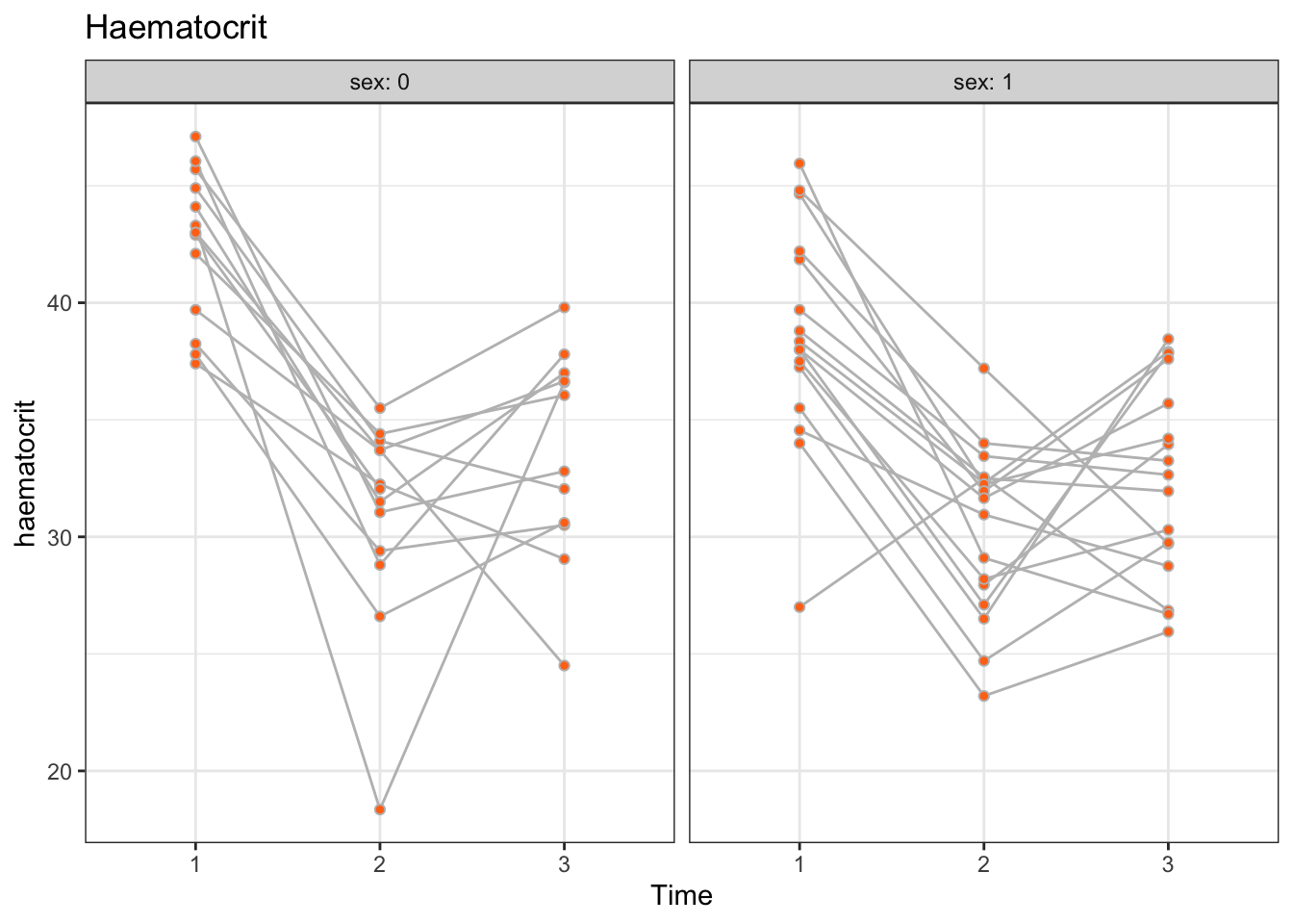
There appears to be heterogeneity between patients for both males and females. We observe no profound differences in profiles between males and females, perhaps apart from males having slightly elevated haematocrit levels. Also, with a few exceptions, the profiles appear to be roughly parallel across patients, or, equivalently, there appears to be no substantial heterogeneity in time.
Let’s fit all possible nested models of the model that includes an interaction of sex with age and time for the fixed effects, and random effects for patient, time or both patient and time, and compute the AIC and BIC for each model. In doing so, we need to respect marginality constraints. In other words, the list of candidate models should include all possible models with main effects (2^3 = 8 in that case), and from the models with interactions we should include only those that include their respective main effects. We can easily list the resulting set of candidate models for the fixed-effects in that case:
We can now include the above model formulas in R in a list, after adding a random intercept for patient, and use a for loop to fit all models using lmer() with REML = FALSE, and compute AIC, BIC and AICc for each model.
The code chunk below does that for AIC, BIC, and AICc.
We see that AIC and AICc agree that the best model is the model with main effects for sex and time and a patient-specific random intercept. That model is only second-best in terms of BIC (BIC of 522.01) after the model with with a main effect of only time (BIC of 520.81).
So, from the models with patient-specific intercepts, there is evidence for the model y ~ sex + time + (1 | subj).
We get an error message, because there are now too many different random effect terms in the model to be able to estimate them all from the data available.
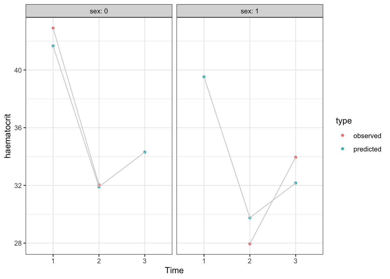
In order to identify the patients with missing haematocrit measurements, we check which patients do not have all 3 times in the data.
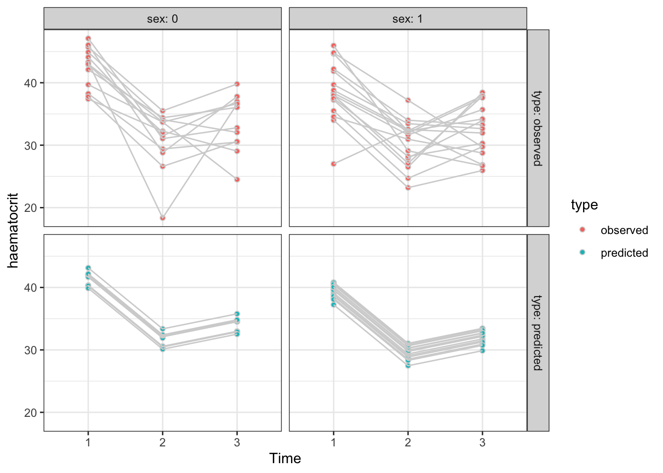
Since the chosen model only involves sex, time and subject, we want to predict the haematocrit levels for every row of the data frame
Akaike, H. (1973). Information theory and an extension of the maximum likelihood principle. In B. N. Petrov & F. Czáki (Eds.),
Second international symposium on information theory (pp. 267–281). Akad
emiai Kiad
ó.
https://doi.org/10.1007/978-1-4612-0919-5_38
Albert, J. H. (2007).
Bayesian computation with r. Springer-Verlag.
https://doi.org/10.1007/978-0-387-92298-0
Albert, J. H., & Chib, S. (1993). Bayesian analysis of binary and polychotomous response data.
Journal of the American Statistical Association,
88, 669–679.
https://doi.org/10.2307/2290350
Best, N., & Thomas, A. (2000). Bayesian graphical models and software for
GLMs. In D. K. Dey, S. K. Ghosh, & B. K. Mallick (Eds.),
Generalized linear models: A Bayesian perspective (pp. 387–406). Marcel Dekker.
https://doi.org/10.1201/9781482293456
Breslow, N. E., & Clayton, D. G. (1993). Appproximate inference in generalised linear mixed models.
Journal of the American Statistical Association,
88, 9–25.
https://doi.org/10.2307/2290687
Burnham, K. P., & Anderson, D. R. (2002).
Model selection and multi-model inference: A practical information theoretic approach (Second). Springer.
https://doi.org/10.1007/978-1-4757-2917-7
Candès, E., & Tao, T. (2007). The
Dantzig selector: Statistical estimation when
\(p\) is much larger than
\(n\) (with discussion).
Annals of Statistics,
35, 2313–2404.
https://doi.org/10.1214/009053606000001523
Claeskens, G., & Hjort, N. L. (2008).
Model selection and model averaging. Cambridge University Press.
https://doi.org/10.1017/CBO9780511790485
Cowell, R. G., Dawid, A. P., Lauritzen, S. L., & Spiegelhelter, D. J. (1999).
Probabilistic networks and expert systems. Springer-Verlag.
https://doi.org/10.1007/b97670
Crowder, M. J., & Hand, D. J. (1990).
Analysis of repeated measures. Chapman; Hall/CRC.
https://doi.org/10.1201/9781315137421
Davison, A. C. (2003).
Statistical models. Cambridge University Press.
https://doi.org/10.1017/CBO9780511815850
Dempster, A. P., Laird, N. M., & Rubin, D. B. (1977). Maximum likelihood from incomplete data via the
EM algorithm (with discussion).
Journal of the Royal Statistical Society Series B,
39, 1–38.
https://doi.org/10.1111/j.2517-6161.1977.tb01600.x
Diggle, P. J., Heagerty, P., Liang, K.-Y., & Zeger, S. (2002).
Analysis of longitudinal data (2nd ed.). Oxford University Press.
https://global.oup.com/academic/product/analysis-of-longitudinal-data-9780199676750
Draper, D. (1995). Assessment and propagation of model uncertainty (with discussion).
Journal of the Royal Statistical Society Series B,
57, 45–97.
https://doi.org/10.1111/j.2517-6161.1995.tb02015.x
Efron, B. (1975). Defining the curvature of a statistical problem (with applications to second order efficiency).
The Annals of Statistics,
3(6), 1189–1242.
https://doi.org/10.1214/aos/1176343282
Fahrmeir, L., Kneib, T., Lang, S., & Marx, B. (Eds.). (2013).
Regression: Models, methods and applications. Springer.
https://doi.org/10.1007/978-3-642-34333-9
Fan, J., & Li, R. (2001). Variable selection via nonconcave penalized likelihood and its oracle properties. Journal of the American Statistical Association, 96, 1348–1360.
Fan, J., & Lv, J. (2008). Sure independence screening for ultrahigh dimensional feature space (with
Discussion).
Journal of the Royal Statistical Society Series B,
70, 849–911.
https://doi.org/10.1198/016214501753382273
Gelman, A., Carlin, J. B., Stern, H. S., Dunson, D. B., Vehtari, A., & Rubin, D. B. (2004).
Bayesian data analysis (3rd ed.). Chapman; Hall/CRC.
https://doi.org/10.1201/b16018
Gelman, A., Hill, J., & Vehtari, A. (2020).
Regression and other stories. Cambridge University Press.
https://doi.org/10.1017/9781139161879
Gilks, W. R., Richardson, S., & Spiegelhalter, D. J. (Eds.). (1996). Markov chain monte carlo in practice. Chapman & Hall.
Green, P. J., Hjørt, N. L., & Richardson, S. (Eds.). (2003).
Highly structured stochastic systems. Chapman & Hall/CRC.
10.1201/b14835
Hastie, T., Tibshirani, R., & Wainwright, M. (2015).
Statistical learning with sparsity: The Lasso and generalizations. Chapman; Hall/CRC.
https://doi.org/10.1201/b18401
Hoeting, J. A., Madigan, D., Raftery, A. E., & Volinsky, C. T. (1999). Bayesian model averaging: A tutorial (with discussion).
Statistical Science,
14, 382–417.
https://doi.org/10.1214/ss/1009212519
Jamshidian, M., & Jennrich, R. I. (1997). Acceleration of the
EM algorithm by using quasi-
Newton methods.
Journal of the Royal Statistical Society Series B,
59, 569–587.
https://doi.org/10.1111/1467-9868.00083
Kass, R. E., & Raftery, A. E. (1995). Bayes factors.
Journal of the American Statistical Association,
90, 773–795.
https://doi.org/10.1080/01621459.1995.10476572
Liang, K., & Zeger, S. L. (1986). Longitudinal data analysis using generalized linear models.
Biometrika,
73(1), 13–22.
https://doi.org/10.1093/biomet/73.1.13
Linhart, H., & Zucchini, W. (1986).
Model selection. Wiley.
https://doi.org/10.1007/978-3-642-04898-2_373
Little, R. J. A., & Rubin, D. B. (2002).
Statistical analysis with missing data (2nd ed.). Wiley.
https://doi.org/10.1002/9781119013563
Marin, J.-M., & Robert, C. P. (2007).
Bayesian core: A practical approach to computational bayesian statistics. Springer-Verlag.
https://doi.org/10.1007/978-0-387-38983-7
McCullagh, P. (2002). What is a statistical model?
The Annals of Statistics,
30(5), 1225–1310.
https://doi.org/10.1214/aos/1035844977
McCullagh, P., & Nelder, J. A. (1989).
Generalized linear models (2nd ed.). Chapman & Hall.
https://doi.org/10.1201/9780203753736
McCulloch, C. E., Searle, S. R., & Neuhaus, J. M. (2008).
Generalized, linear, and mixed models (2nd ed.). Wiley.
https://doi.org/10.1002/0471722073
McLachlan, G. J., & Krishnan, T. (2008).
The EM algorithm and extensions (2nd ed.). Wiley.
https://doi.org/10.1002/9780470191613
McQuarrie, A. D. R., & Tsai, C.-L. (1998).
Regression and time series model selection. World Scientific.
https://doi.org/10.1142/3573
Meng, X.-L., & van Dyk, D. (1997). The
EM algorithm — an old folk-song sung to a fast new tune (with discussion).
Journal of the Royal Statistical Society Series B,
59, 511–567.
https://doi.org/10.1111/1467-9868.00082
Nelder, J. A., Lee, Y., & Pawitan, Y. (2017).
Generalized linear models with random effects: A unified approach via \(h\)-likelihood (2nd ed.). Chapman; Hall/CRC.
https://doi.org/10.1201/9781315119953
Nelder, J. A., & Wedderburn, R. W. M. (1972). Generalized linear models.
Journal of the Royal Statistical Society: Series A (General),
135(3), 370–384.
https://doi.org/10.2307/2344614
O’Hagan, A., & Forster, J. J. (2004).
Kendall’s advanced theory of statistics. Volume 2B: Bayesian inference (Second). Hodder Arnold.
https://www.wiley.com/en-us/Kendall%27s+Advanced+Theory+of+Statistic+2B-p-9780470685693
Oakes, D. (1999). Direct calculation of the information matrix via the
EM algorithm.
Journal of the Royal Statistical Society Series B,
61, 479–482.
https://doi.org/10.1111/1467-9868.00188
Ogden, H. (2021). On the error in laplace approximations of high-dimensional integrals.
Stat,
10(1), e380.
https://doi.org/10.1002/sta4.380
Ogden, H. E. (2017). On asymptotic validity of naive inference with an approximate likelihood.
Biometrika,
104(1), 153–164.
https://doi.org/10.1093/biomet/asx002
Peters, J., Janzing, D., & Schlkopf, B. (2017).
Elements of causal inference: Foundations and learning algorithms. The MIT Press.
https://mitpress.mit.edu/books/elements-causal-inference
Pinheiro, J., & Bates, D. M. (2002).
Mixed effects models in S and S-PLUS. New York:Springer-Verlag.
https://doi.org/10.1007/b98882
Raftery, A. E., Madigan, D., & Hoeting, J. A. (1997). Bayesian model averaging for linear regression models.
Journal of the American Statistical Association,
92, 179–191.
https://doi.org/10.1080/01621459.1997.10473615
Richardson, S., & Green, P. J. (1997). On bayesian analysis of mixtures with an unknown number of components (with discussion).
Journal of the Royal Statistical Society Series B,
59, 731–792.
https://doi.org/10.1111/1467-9868.00095
Rissanen, J. (1987). Stochastic complexity (with discussion).
Journal of the Royal Statistical Society, Series B,
49, 223–239.
https://doi.org/10.1111/j.2517-6161.1987.tb01694.x
Schwartz, G. (1978). Estimating the dimension of a model.
Annals of Statistics,
6, 461–464.
https://doi.org/10.1214/aos/1176344136
Spiegelhalter, D. J., Best, N. G., Carlin, B. P., & Linde, A. van der. (2002). Bayesian measures of model complexity and fit (with discussion).
Journal of the Royal Statistical Society, Series B,
64, 583–639.
https://doi.org/10.1111/1467-9868.00353
Tanner, M. A. (1996).
Tools for statistical inference: Methods for the exploration of posterior distributions and likelihood functions (Third). Springer.
https://doi.org/10.1007/978-1-4612-4024-2
Venables, W., & Ripley, B. D. (2002).
Modern applied statistics with S (4th ed.). Springer-Verlag.
https://doi.org/10.1007/978-0-387-21706-2
Wedderburn, R. W. M. (1974). Quasi-
Likelihood Functions,
Generalized Linear Models, and the
Gauss-Newton Method.
Biometrika,
61(3), 439.
https://doi.org/10.2307/2334725
Wood, S. N. (2017).
Generalized additive models: An introduction with r (2nd ed.). Chapman; Hall/CRC.
https://doi.org/10.1201/9781315370279