We must be careful not to confuse data with the abstractions we use to analyse them.
— William James (1842 – 1910)
2.1 Generalized linear models
Suppose that \(y_1, \ldots, y_n\) are observations of response variables \(Y_1, \ldots, Y_n\), which are assumed to be independent conditionally on covariates \(x_1, \ldots, x_n\). Furthermore, assume that \(Y_i\) has an exponential family distribution. A generalized linear models links the mean \(\mu_i = \mathop{\mathrm{E}}(Y_i \mid x_i)\) to a linear combination of covariates and regression parameters through a link function \(g(\cdot)\) as \[
g(\mu_i) = \eta_i = x_i^\top \beta \, .
\]
Generalized linear models (GLMs) have proved effective at modelling real-world variation in a wide range of application areas. However, situations frequently arise where GLMs do not adequately describe observed data. This can be due to a number of reasons including:
The mean model cannot be appropriately specified due to dependence on an unobserved or unobservable covariate.
There is excess variability between experimental units beyond what is implied by the mean/variance relationship of the chosen response distribution.
The assumption of independence is not appropriate.
Complex multivariate structures in the data require a more flexible model.
2.2 Overdispersion
An example
Example 2.1 (Toxoplasmosis data) The toxo dataset in the SMPracticals R package provides data on the number of people testing positive for toxoplasmosis (r) out of the number of people tested (m) in 34 cities in El Salvador, along with the annual rainfall in mm (rain) in those cities.
We consider logistic regression models that assume that the numbers \(r_1, \ldots, r_{n}\) of people testing positive for toxoplasmosis in the \(n = 34\) cities are realizations of independent random variables \(R_1, \ldots, R_n\), conditionally on a function of the annual rainfall \(x_i\), and that \(R_i \mid x_i \sim \mathop{\mathrm{Binomial}}(m_i, \mu_i)\), where \[
\log \frac{\mu_i}{1 - \mu_i} = \eta_i = \beta_1 + f(x_i) \, .
\]
Let \(Y_i = R_i / m_i\) be the proportion of people testing positive in the \(i\)th city. Because of the assumption of a binomial response distribution, a logistic regression model sets the response variance to \(\mathop{\mathrm{var}}(Y_i \mid
x_i) = \mu_i (1 - \mu_i) / m_i\).
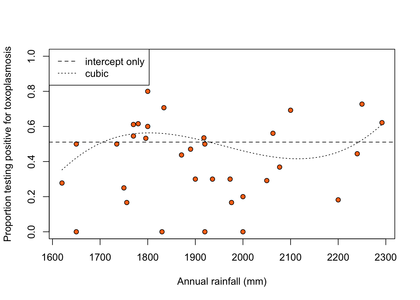
If we consider logistic models with a linear predictor that implies a polynomial dependence on rainfall, AIC and stepwise selection methods both prefer a cubic model. For simplicity here, we compare a cubic model and an intercept-only model, in which there is no dependence on rainfall. Figure 2.1 shows the fitted proportions testing positive under the two models.
Figure 2.1: Proportion of people testing positive for toxoplasmosis against rainfall, with fitted proportions under an intercept-only (dashed line) and a cubic (dotted line) logistic regression model.
We can also compare the models using a hypothesis test:
There is evidence against the intercept-only model, which implies no effect of rain on the probability of testing positive for toxoplasmosis, in favour of the cubic model.
However, we find that the residual deviance for the cubic model is 62.63, which is much larger than the residual degrees of freedom (30). That is evidence of a poor fit, and may be due to overdispersion of the responses. Overdispersion results in the residual variability being greater than what is prescribed by the mean / variance relationship of logistic regression.
Quasi-likelihood
A quasi-likelihood approach to accounting for overdispersion models the mean and variance, but stops short of a full probability model for the responses.
For a model specified by the mean relationship \(g(\mu_i) = \eta_i\), and variance \(\mathop{\mathrm{var}}(Y_i \mid x_i) = \sigma^2 V(\mu_i) / m_i\), the quasi-likelihood equations are \[
\sum_{i = 1}^n x_i {\frac{y_i-\mu_i}{\sigma^2 V(\mu_i) g'(\mu_i)/m_i}} = 0 \, ,
\tag{2.1}\] which can be solved with respect to \(\beta\) without knowledge of \(\sigma^2\).
If \(V(\mu_i)\) is the same function as in the definition of \(\mathop{\mathrm{var}}(Y_i
\mid x_i)\) for an exponential family distribution, then it may be possible to solve (2.1) using standard GLM routines.
It can be shown that provided the mean and variance functions are correctly specified, asymptotic normality for \(\hat\beta\) still holds.
The dispersion parameter \(\sigma^2\) can be estimated after estimating \(\beta\), as \[
\hat\sigma^2\equiv \frac{1}{n - p} \sum_{i=1}^n \frac{m_i(y_i-\hat{\mu}_i)^2}{V(\hat{\mu}_i)} \, .
\]
Example 2.2 (Quasi-likelihood for the toxoplasmosis data) In order to fit the same models as before, but with \(\mathop{\mathrm{var}}(Y_i \mid x_i) = \sigma^2 \mu_i (1 - \mu_i) / m_i\), we do
Code
mod_const_quasi <-glm(r/m ~1, data = toxo, weights = m,family ="quasibinomial")mod_cubic_quasi <-glm(r/m ~poly(rain, 3), data = toxo, weights = m,family ="quasibinomial")
Comparing the output from fitting the logistic regression with a cubic relationship to rainfall
Code
summary(mod_cubic)
Call:
glm(formula = r/m ~ poly(rain, 3), family = "binomial", data = toxo,
    weights = m)

Coefficients:
               Estimate Std. Error z value Pr(>|z|)
(Intercept)     0.02427    0.07693   0.315 0.752401
poly(rain, 3)1 -0.08606    0.45870  -0.188 0.851172
poly(rain, 3)2 -0.19269    0.46739  -0.412 0.680141
poly(rain, 3)3  1.37875    0.41150   3.351 0.000806 ***
---
Signif. codes:  0 '***' 0.001 '**' 0.01 '*' 0.05 '.' 0.1 ' ' 1

(Dispersion parameter for binomial family taken to be 1)

    Null deviance: 74.212  on 33  degrees of freedom
Residual deviance: 62.635  on 30  degrees of freedom
AIC: 161.33

Number of Fisher Scoring iterations: 3
to the corresponding output from solving the quasi-likelihood equations
Code
summary(mod_cubic_quasi)
Call:
glm(formula = r/m ~ poly(rain, 3), family = "quasibinomial",
    data = toxo, weights = m)

Coefficients:
               Estimate Std. Error t value Pr(>|t|)
(Intercept)     0.02427    0.10716   0.226   0.8224
poly(rain, 3)1 -0.08606    0.63897  -0.135   0.8938
poly(rain, 3)2 -0.19269    0.65108  -0.296   0.7693
poly(rain, 3)3  1.37875    0.57321   2.405   0.0225 *
---
Signif. codes:  0 '***' 0.001 '**' 0.01 '*' 0.05 '.' 0.1 ' ' 1

(Dispersion parameter for quasibinomial family taken to be 1.940446)

    Null deviance: 74.212  on 33  degrees of freedom
Residual deviance: 62.635  on 30  degrees of freedom
AIC: NA

Number of Fisher Scoring iterations: 3
we observe that the estimates of the \(\beta\) coefficients are the same, but the estimated standard errors from quasi-likelihood are inflated by a factor of 1.39, which is equal to the square root of the estimate \(\hat\sigma^2 = 1.94\) of \(\sigma^2\). Note that the value of \(\hat\sigma^2\) is about double than \(\sigma^2 = 1\), implied by logistic regression.
A comparison of two quasi-likelihood fits is usually performed by mimicking the \(F\) test for nested linear regression models, using residual deviances in place of residual sums of squares. The resulting \(F\) statistic is asymptotically valid. To illustrate, we compare the value of \(F\) statistic \[
F = \frac{(74.21 - 62.63) / (33 - 30)}{1.94} \, ,
\] to quantiles of its asymptotic \(F\) distribution with 33 - 30 and 30 degrees of freedom. In R, we get
Code
anova(mod_const_quasi, mod_cubic_quasi, test ="F")
Analysis of Deviance Table

Model 1: r/m ~ 1
Model 2: r/m ~ poly(rain, 3)
  Resid. Df Resid. Dev Df Deviance      F Pr(>F)
1        33     74.212
2        30     62.635  3   11.577 1.9888 0.1369
After accounting for overdispersion, the evidence in favour of an effect of rainfall on toxoplasmosis incidence is less compelling.
Parametric models for overdispersion
To construct a full probability model in the presence of overdispersion, it is necessary to consider the reasons for the presence of overdispersion. Possible reasons include:
There may be important covariates, other than rainfall, which are not observed.
There may be many other features of the cities, possibly unobservable, all having a small individual effect on incidence, but a larger effect in combination. Such effects may be individually undetectable, a phenomenon sometimes described as natural excess variability between units.
Suppose that part of the linear predictor is missing from the model, that is the actual predictor is \[
\eta_i^* = \eta_i + \zeta_i \,,
\] instead of just \(\eta_i\), where \(\zeta_i\) may involve covariates \(z_i\) that are different than those in \(x_i\). We can compensate for the missing term \(\zeta_i\) by assuming that it has a distribution \(F\) in the population. Hence, \[
\mu_i = \mathop{\mathrm{E}}(Y_i \mid x_i, \zeta_i) = g^{-1}(\eta_i + \zeta_i)\sim G \, ,
\] where \(G\) is the distribution induced by \(F\). Then, \[
\begin{aligned}
\mathop{\mathrm{E}}(Y_i \mid x_i) & = {\mathop{\mathrm{E}}}_G(\mu_i) \, ,\\
\mathop{\mathrm{var}}(Y_i \mid x_i) & = {\mathop{\mathrm{E}}}_G( \mathop{\mathrm{var}}(Y_i \mid x_i, \zeta_i) ) + {\mathop{\mathrm{var}}}_G(\mu_i) \, .
\end{aligned}
\] For exponential family models, we get \(\mathop{\mathrm{var}}(Y_i \mid x_i) = \sigma^2 {\mathop{\mathrm{E}}}_G(
V(\mu_i)) / m_i + {\mathop{\mathrm{var}}}_G(\mu_i)\).
One approach is to model the \(Y_i\) directly, by specifying an appropriate form for \(G\). For example, for the toxoplasmosis data, instead of a quasi-likelihood approach, we can use a beta-binomial model, where \[
\begin{aligned}
Y_i & = R_i / m_i \,, \\
R_i \mid \mu_i & \stackrel{\text{ind}}{\sim}\mathop{\mathrm{Binomial}}(m_i, \mu_i) \,, \\
\mu_i \mid x_i & \stackrel{\text{ind}}{\sim}\mathop{\mathrm{Beta}}(k \mu^*_i, k (1 - \mu^*_i)) \,, \\
\log \{ \mu_i^* / (1 - \mu_i^*) \} & = \eta_i \,,
\end{aligned}
\] leading to \[
\mathop{\mathrm{E}}(Y_i \mid x_i) = \mu^*_i \quad \text{and} \quad
\mathop{\mathrm{var}}(Y_i \mid x_i) = \frac{\mu^*_i (1-\mu^*_i)}{m_i} \left(1 + \frac{m_i - 1}{k + 1}\right) \,,
\] with \((m_i - 1)/(k + 1)\) representing the overdispersion factor.
Another, popular in practice, model that accounts for overdispersion in count responses assumes a Poisson distribution for the responses and that the Poisson mean has a gamma distribution. This leads to a negative binomial marginal distribution for the responses.
Models that explicitly account for overdispersion can, in principle, be fitted with popular estimation methods, such as maximum likelihood. For example, the beta-binomial model has likelihood proportional to \[
\prod_{i = 1}^n \frac{\Gamma(k\mu_i^* + m_i y_i)
\Gamma(k (1 - \mu_i^*) + m_i (1 - y_i)) \Gamma(k)}{
\Gamma(k\mu_i^*)\Gamma(k ( 1 - a\mu_i^*))\Gamma(k + m_i)} \,.
\]
However, these models tend to have limited flexibility, and maximization of the likelihood can be difficult. For those reasons, practitioners typically resort to alternative approaches.
A more flexible, and extensible approach models the excess variability by including an extra term in the linear predictor \[
\eta_i = x_i^\top\beta + b_i
\tag{2.2}\] where \(b_1, \ldots, b_n\) can be thought of as representing the extra, unexplained by the covariates, variability between units, and are called random effects. The model is completed by specifying a distribution \(F\) for the random effects in the population. A typical assumption is that \(b_1, \ldots, b_n\) are independent with \(b_i \sim
{\mathop{\mathrm{N}}}(0,\sigma^2_b)\), for some unknown \(\sigma^2_b\). We set \(\mathop{\mathrm{E}}(b_i) = 0\), as an unknown mean for \(b_i\) would be unidentifiable in the presence of the intercept parameter in \(\eta_i\).
Let \(f(y_i \mid x_i, b_i \,;\,\theta)\) be the density or probability mass function of the chosen exponential family distribution, with linear predictor (2.2), and \(f(b_i \mid \sigma^2_b)\) the density function of a univariate normal distribution with mean \(0\) and variance \(\sigma^2_b\). The likelihood about the parameters \((\theta^\top, \sigma^2_b)^\top\) of the random effects model is \[
\begin{aligned}
f(y\mid X \,;\,\theta, \sigma^2_b)&=\int f(y \mid X, b \,;\,\theta, \sigma^2_b)f(b \mid X \,;\,\theta, \sigma^2_b)db\\
&=\int f(y \mid X, b \,;\,\theta)f(b \,;\,\sigma^2_b) db \\
&=\int \prod_{i=1}^n f(y_i \mid x_i, b_i \,;\,\theta) f(u_i \,;\,\sigma^2_b)db_i \, .
\end{aligned}
\tag{2.3}\]
Depending on what \(f(y_i \mid x_i, b_i \,;\,\theta)\) is, no further simplification of (2.3) may be possible, and computation needs careful consideration. We will briefly discuss such points later.
2.3 Dependence
An example
Example 2.3 (Toxoplasmosis data (revisited)) We can think of the toxoplasmosis cases in the \(i\)th city arising as \(R_i = \sum_{j = 1}^{m_i} Y_{ij}\), where \(Y_{ij}\) is a Bernoulli random variable, representing the toxoplasmosis status of individual \(j\), with probability \[
\log \frac{\mu_{ij}}{1 - \mu_{ij}} = \eta_i = \beta_1 + f(x_i) \, .
\tag{2.4}\] From the properties of the binomial distirbution, if \(\{Y_{ij}\}\) are independent, then the logistic regresion model on \(\{R_i\}\) in Example 2.1 is the same to the Bernoulli model on \(\{Y_{ij}\}\). However, suppose that the only assumptions we can confidently make is that \(\{R_i\}\) are conditionally independent given the covariates and that \(\mathop{\mathrm{cov}}(Y_{ij}, Y_{ik} \mid x_i) \ne 0\). Then, \[
\begin{aligned}
\mathop{\mathrm{var}}(Y_i \mid x_i) & = \frac{1}{m_i^2}\left\{\sum_{j=1}^{m_i} \mathop{\mathrm{var}}(Y_{ij} \mid x_i) + \sum_{j \ne k} \mathop{\mathrm{cov}}(Y_{ij}, Y_{ik} \mid x_i)\right\} \\
& = \frac{\mu_i (1 - \mu_i)}{m_i} + \frac{1}{m_i^2} \sum_{j \ne k} \mathop{\mathrm{cov}}(Y_{ij}, Y_{ik} \mid x_i) \, .\\
\end{aligned}
\] As a result, positive correlation between individuals in the same city induces overdispersion in the number of positive cases.
There may be a number of plausible reasons why there is dependence between responses corresponding to units within a given cluster (in the toxoplasmosis example, clusters are cities). One compelling reason, that we discussed already, is unobserved heterogeneity.
In the correct model (corresponding to \(\eta_i^*\)), the toxoplasmosis status of individuals, \(Y_{ij}\), may be independent, so \[
Y_{ij} \perp\!\!\!\perp Y_{ik} \mid x_i, \zeta_i \quad (j \ne k) \,.
\] However, in the absence of knowledge of \(\zeta_i\), it may be the case that \[
Y_{ij} \perp\!\!\!\perp\!\!\!\!\!\!/\;\;Y_{ik} \mid x_i \quad (j \ne k)\, .
\]
Hence conditional (given \(\zeta_i\)) independence between units in a common cluster \(i\) becomes marginal dependence, when marginalised over the population distribution \(F\) of unobserved \(\zeta_i\).
The correspondence between positive intra-cluster correlation and unobserved heterogeneity suggests that intra-cluster dependence might be effectively modelled using random effects. For example, for the individual-level toxoplasmosis data \[
\begin{aligned}
Y_{ij} \mid x_{i}, b_i & \stackrel{\text{ind}}{\sim}\mathop{\mathrm{Bernoulli}}(\mu_{ij}) \,, \\
\log \frac{\mu_{ij}}{1-\mu_{ij}} & = \beta_1 + f(x_i) + b_i\,, \\
b_i & \stackrel{\text{ind}}{\sim}{\mathop{\mathrm{N}}}(0, \sigma^2_b)\,,
\end{aligned}
\] which, for \(\sigma^2 > 0\), implies \[
Y_{ij} \perp\!\!\!\perp\!\!\!\!\!\!/\;\;Y_{ik} \mid x_{i} \, .
\]
Intra-cluster dependence arises in many applications, and random effects provide an effective way of modelling it.
Marginal models
Another way to account for intra-cluster dependence are marginal models. A marginal model expresses \(\mu_{ij} = \mathop{\mathrm{E}}(Y_{ij} \mid
\eta_{ij})\) as a function of explanatory variables, through \(g(\mu_{ij}) = \eta_{ij} = x_{ij}^\top \beta\), specifies a variance relationship \(\mathop{\mathrm{var}}(Y_{ij} \mid x_{ij})= \sigma^2 V(\mu_{ij}) /
m_{ij}\), and models \(\mathop{\mathrm{corr}}(Y_{ij}, Y_{ik} \mid x_{ij}, x_{ik})\), as a function of \(\mu\) and possibly additional parameters.
It is important to note that the parameters \(\beta\) in a marginal model have a different interpretation from those in a random effects model, because for the latter \[
\mathop{\mathrm{E}}(Y_{ij} \mid x_{ij}) = \mathop{\mathrm{E}}(g^{-1}[x_{ij}^\top \beta + b_i]) \ne g^{-1}(x_{ij}^\top \beta) \quad \text{if $g$ is not linear} \,.
\]
A random effects model describes the mean response at the subject level (subject specific), while a marginal model describes the mean response across the population (population averaged).
As with the quasi-likelihood approach above, marginal models do not generally provide a full probability model for the responses. Nevertheless, \(\beta\) can be estimated using generalized estimating equations (GEEs).
The GEE estimator of $ in a marginal model is the solution of of the form \[
\sum_i \left(\frac{\partial\mu_i}{\partial\beta}\right)^\top \mathop{\mathrm{var}}(Y_i)^{-1}(Y_i-\mu_i) = 0 \,,
\] where \(Y_i = (Y_{i1}, \ldots, Y_{in_i})^\top\) and \(\mu_i = (\mu_{i1},
\ldots, \mu_{in_i})^\top\), with \(n_i\) indicating the number of observations in the \(i\)th response vector.
There are several consistent estimators for the covariance of GEE estimators. Furthermore, the GEE approach is generally robust to misspecification of the correlation structure.
Clustered data
Examples where data are collected in clusters include:
Studies in biometry where repeated measurements are made on experimental units. Such studies can effectively mitigate the effect of between-unit variability on important inferences.
Agricultural field trials, or similar studies, for example in engineering, where experimental units are arranged within blocks.
Sample surveys where collecting data within clusters or small areas can save costs.
Of course, other forms of dependence exist, for example spatial or serial dependence induced by the arrangement of units of observation in space or time.
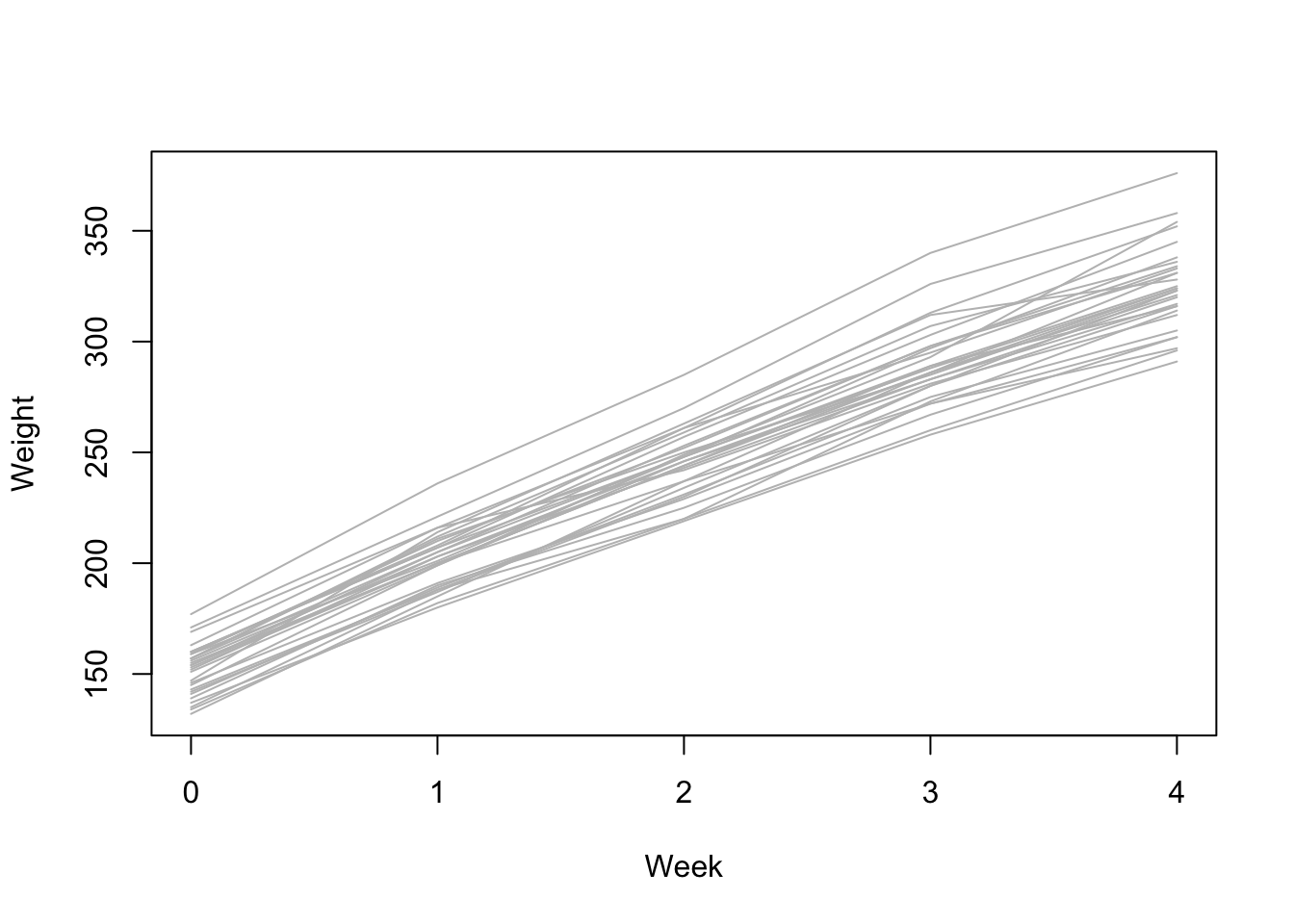
Example 2.4 The rat.growth data in the SMPracticals R package gives the weekly weights (y) of 30 young rats. Figure 2.2 shows the weight evolution for each rat. While the weights of each rat appears to grow roughly linearly with time, the intercept and slope of that weight evolution seem to vary between rats.
Code
data("rat.growth", package ="SMPracticals")plot(y ~ week, data = rat.growth, type ="n", xlab ="Week", ylab ="Weight")for (i in1:30) { dat_i <-subset(rat.growth, rat == i)lines(y ~ week, data = dat_i, col ="grey")}
Figure 2.2: Individual rat weight by week, for the rat growth data.
Writing \(y_{ij}\) for the weight of rat \(i\) at week \(x_{ij}\), we consider the simple linear regression \[
Y_{ij} = \beta_1 + \beta_2 x_{ij} + \epsilon_{ij} \, ,
\] and fit it using R:
Code
rat_lm <-lm(y ~ week, data = rat.growth)(rat_lm_sum <-summary(rat_lm))
Call:
lm(formula = y ~ week, data = rat.growth)

Residuals:
   Min     1Q Median     3Q    Max
-38.12 -11.25   0.28   7.68  54.15

Coefficients:
            Estimate Std. Error t value Pr(>|t|)
(Intercept)  156.053      2.246   69.47   <2e-16 ***
week          43.267      0.917   47.18   <2e-16 ***
---
Signif. codes:  0 '***' 0.001 '**' 0.01 '*' 0.05 '.' 0.1 ' ' 1

Residual standard error: 15.88 on 148 degrees of freedom
Multiple R-squared:  0.9377,    Adjusted R-squared:  0.9372
F-statistic:  2226 on 1 and 148 DF,  p-value: < 2.2e-16
The resulting estimates are \(\hat\beta_1= 156.05\) and \(\hat\beta_2 = 43.27\), with estimated standard errors \(2.25\) and \(0.92\), respectively.
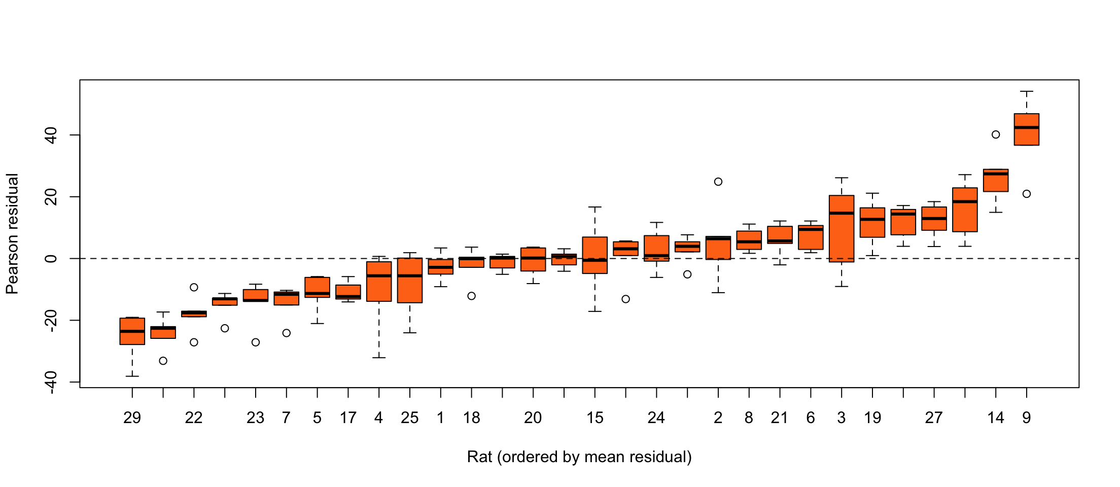
Figure 2.3 shows boxplots of the residuals from this model, separately for each rat. There is clear evidence of unexplained differences between rats.
Code
res <-residuals(rat_lm, type ="pearson")ord <-order(ave(res, rat.growth$rat))rats <- rat.growth$rat[ord]rats <-factor(rats, levels =unique(rats), ordered =TRUE)plot(res[ord] ~ rats,xlab ="Rat (ordered by mean residual)",ylab ="Pearson residual",col ="#ff7518", pch =21)abline(h =0, lty =2)
Figure 2.3: Boxplots of residuals from a simple linear regression, for each rat in the rat growth data.
2.4 Linear mixed models
Model definition
A linear mixed model (LMM) for observations \(y = (y_1, \ldots , y_n)^\top\) has the general form \[
\begin{aligned}
Y \mid X, Z, b & \sim {\mathop{\mathrm{N}}}(\mu, \Sigma) \,, \\
\mu & = X\beta + Z b \, , \\
b & \sim {\mathop{\mathrm{N}}}(0, \Sigma_b) \,.
\end{aligned}
\tag{2.5}\] where \(X\) and \(Z\) are matrices containing covariate values. Usually, \(\Sigma = \sigma^2 I_n\). The unknown parameters to be estimated are \(\beta\), \(\Sigma\), and \(\Sigma_b\). The term mixed model highlights that the linear predictor \(X\beta + Z b\) contains both the fixed effects \(\beta\) and the random effects \(b\).
A typical example for clustered data is \[
\begin{aligned}
Y_{ij} \mid x_{ij}, z_{ij}, b_i & \stackrel{\text{ind}}{\sim}{\mathop{\mathrm{N}}}(\mu_{ij},\sigma^2) \,, \\
\mu_{ij} & = x_{ij}^\top \beta + z_{ij}^\top b_i \,, \\
b_i & \stackrel{\text{ind}}{\sim}{\mathop{\mathrm{N}}}(0,\Sigma^*_b) \,,
\end{aligned}
\tag{2.6}\] where \(x_{ij}\) contains the covariates for observation \(j\) of the \(i\)th cluster, and \(z_{ij}\) the covariates which are allowed to exhibit extra between-cluster variation in their relationship with the response. Typically, \(z_{ij}\) is a sub-vector of \(x_{ij}\), but this is not necessary.
The simplest case of a mixed effects linear predictor arises when \(z_{ij} = 1\), which results in a random-intercept model, as in (2.2).
A plausible LMM for \(k\) clusters with \(n_i\) observations in the \(i\)th cluster, and a single explanatory variable (see, for example, Example 2.4) has \[
Y_{ij} = \beta_1 + b_{1i} + (\beta_2 + b_{2i}) x_{ij} + \epsilon_{ij}\,,\quad
(b_{1i},b_{2i})^\top \stackrel{\text{ind}}{\sim}{\mathop{\mathrm{N}}}(0, \Sigma^*_b)\,.
\]
This fits into the general LMM definition in (2.5) with \(\Sigma = \sigma^2 I_n\), and \[
Y = \begin{bmatrix}
Y_1 \\
\vdots \\
Y_k
\end{bmatrix}\,, \quad
Y_i = \begin{bmatrix}
Y_{i1} \\
\vdots \\
Y_{in_i}
\end{bmatrix} \, ,
\]\[
X = \begin{bmatrix}
X_1 \\
\cdots \\
X_k
\end{bmatrix}\,, \quad
Z = \begin{bmatrix}
X_1 & 0 & \cdots & 0 \\
0 & X_2 & \cdots & 0 \\
\vdots & \vdots & \ddots & \vdots \\
0 & 0 & \cdots & X_k
\end{bmatrix}\,, \quad
X_i = \begin{bmatrix}
1 & x_{i1} \\
\vdots & \vdots \\
1 & x_{in_i}
\end{bmatrix}\,,
\]\[
\beta = \begin{bmatrix}
\beta_1 \\
\beta_2
\end{bmatrix}\,, \quad
b = \begin{bmatrix}
b_{11} \\
b_{21} \\
\vdots \\
b_{1k} \\
b_{2k}
\end{bmatrix}\,, \quad
\Sigma_b = \begin{bmatrix}
\Sigma^*_b & 0 & 0 \\
0 & \ddots & 0 \\
0 & 0 & \Sigma^*_b
\end{bmatrix} \, ,
\] where \(\Sigma^*_b\) is an unknown \(2\times 2\) positive definite matrix, and \(0\) denotes a matrix of zeros of appropriate dimension.
Under an LMM, we can write the marginal distribution of \(Y\) directly as \[
Y \mid X, Z \sim {\mathop{\mathrm{N}}}(X \beta,\Sigma + Z\Sigma_b Z^\top )
\tag{2.7}\] Hence, \(\mathop{\mathrm{var}}(Y \mid X, Z)\) is comprised of two variance components.
LMMs for clustered data, such as (2.6) are also known as hierarchical or multilevel models. This reflects the two-stage structure of the model definition; a conditional model for the responses given covariates and the random effects, followed by a marginal model for the random effects.
Sometimes the hierarchy can have further levels, corresponding to clusters nested within clusters. Common practical settings of that kind is patients within wards within hospitals, or pupils within classes within schools.
Random effects or cluster-specific fixed effects
Instead of including random effects for clusters, e.g. \[
Y_{ij} = \beta_1 + b_{1i} + (\beta_2 + b_{2i})x_{ij} +\epsilon_{ij} \, ,
\] we could use separate fixed effects for each cluster, e.g. \[
Y_{ij} = \beta_{1i} + \beta_{2i} x_{ij} + \epsilon_{ij} \,.
\] However, inferences can then only be made about those clusters present in the observed data. Random effects models allow inferences to be extended to a wider population. It also can be the case that fixed effects are not identifiable. That is the case in the setting of Example 2.1 where there is only one observation per cluster. In contrast, random effects are identifiable and can be estimated. Random effects also allow borrowing strength across clusters by shrinking fixed effects towards a common mean.
Estimation
The likelihood about \(\beta\), \(\Sigma\), \(\Sigma_b\) is available from (2.7) as \[
f(y \mid X, Z \,;\,\beta, \Sigma, \Sigma_b) \propto |V|^{-1/2}
\exp\left(-\frac{1}{2} (y-X\beta)^\top V^{-1} (y-X\beta)\right)
\tag{2.8}\] where \(V = \Sigma + Z\Sigma_b Z^\top\), and can be directly maximized.
However, the maximum likelihood estimators for the variance parameters of LMMs can have considerable downward bias. The bias is more profound in cluster models with a small number of observed clusters, and can affect the performance of inferential procedures. Hence estimation by REML (REstricted or REsidual Maximum Likelihood) is usually preferred.
REML proceeds by estimating the variance parameters \(\Sigma\) and \(\Sigma_b\) using a marginal likelihood based on the residuals from a least squares fit of the model \(E(Y \mid X) = X \beta\).
Consider the vector of residuals \((I_n - H) Y\), where \(H = X (X^\top
X)^{-1} X^\top\) is the usual hat matrix. The distribution of \((I_n - H)
Y\) does not depend of \(\beta\), but because \((I_n - H)\) has rank \(n -
p\), that distribution is degenerate. From the spectral decomposition theorem, we can always define a vector of \((n - p)\) random variables \(U = B^\top Y\), where \(B\) is any \(n \times (n - p)\) matrix of rank \((n - p)\) with \(BB^\top = I_n - H\) and \(B^\top B = I_{n - p}\). Then, \(B^\top X = B^\top B B^\top X = B (I_n - H) X = 0\), and \[
\begin{aligned}
U & = B^\top Y = B^\top (X \beta + A) = B^\top A \, , \\
\end{aligned}
\] where \(A \mid Z \sim {\mathop{\mathrm{N}}}(0, V)\). Hence, \(U \mid X, Z \sim \mathop{\mathrm{N}}(0, B^\top V
B)\), which does not depend on \(\beta\). That observation may, at first sight, appear as simply trading the dependence on \(\beta\) with the dependence on \(B\), which would be useless for practical purposes because \(B\) is not uniquely defined. However, it can be shown that the distribution of \(U\) depends neither on \(\beta\) nor on the choice of \(B\)!
To see that, note that the least squares estimator of \(\beta\) for known \(V\) is \[
\hat\beta_V = (X^\top V^{-1} X)^{-1}X^\top V^{-1} Y = \beta + (X^\top V^{-1} X)^{-1}X^\top V^{-1} A \,.
\tag{2.9}\] So, \(\hat\beta_V - \beta \mid X, Z \sim {\mathop{\mathrm{N}}}(0, (X^\top V^{-1} X)^{-1})\). Also, \[
\mathop{\mathrm{E}}(U (\hat\beta_V - \beta)^\top \mid X, Z) = B^\top \mathop{\mathrm{E}}(A A^\top \mid Z) V^{-1} X (X^\top V^{-1}X)^{-1} = 0 \,.
\]
Let \(Q = \begin{bmatrix} B^\top \\ G^\top \end{bmatrix}\), \(G^\top = (X^\top V^{-1} X)^{-1}X^\top V^{-1}\). Then, \[
QY = \begin{bmatrix} U \\ \hat{\beta}_V \end{bmatrix} \,,
\] and \(U\) and \(\hat\beta_V\) have a joint normal distribution. Since they have zero covariance, they are also independent.
Temporarily suppressing the conditioning on \(X\) and \(Z\) in the notation, we can write \[
\begin{aligned}
f(u \,;\,\Sigma, \Sigma_b) f(\hat\beta_V \,;\,\beta, \Sigma, \Sigma_b) & = f(u, \hat\beta_V \,;\,\beta, \Sigma, \Sigma_b) \\
& = f(Q y \,;\,\beta, \Sigma, \Sigma_b) = f(y \,;\,\beta, \Sigma, \Sigma_b) | Q^\top |^{-1} \,,
\end{aligned}
\tag{2.10}\] where \(| Q^\top |\) is the Jacobian determinant of the transformation \(Q y\). We have \[
\begin{aligned}
| Q^\top | & = \left|\begin{bmatrix} B & G \end{bmatrix}\right| \\
& = \left| \begin{bmatrix} B^\top \\ G^\top \end{bmatrix} \begin{bmatrix} B & G \end{bmatrix}\right|^{1/2}
= \left| \begin{bmatrix} B^\top B & B^\top G \\ G^\top B & G^\top G \end{bmatrix} \right|^{1/2} \\
& = |B^\top B|^{1/2} |G^\top G - G^\top B (B^\top B)^{-1} B^\top G|^{1/2} \\
& = |G^\top G - G^\top (I_n - H) G|^{1/2} \\
& = |(X^\top V^{-1} X)^{-1}X^\top V^{-1} X (X^\top X)^{-1} X^\top V^{-1} X (X^\top V^{-1} X)^{-1} |^{1/2} \\
& = |X^\top X|^{-1/2} \, .
\end{aligned}
\] So, from expression (2.10), a completion of the square in the ratio of the normal densities of \(y\) and \(\hat\beta_V\) gives \[
\begin{aligned}
f(u \,;\,\Sigma, \Sigma_b) & = \frac{f(y \,;\,\beta, \Sigma, \Sigma_b)}{f(\hat\beta_V \,;\,\beta, \Sigma, \Sigma_b)} | X^\top X |^{1/2} \\
& \propto \frac{|X^\top X|^{1/2}}{|V|^{1/2} |X^\top V^{-1} X|^{1/2}}
\exp\left(-\frac{1}{2} (y-X\hat\beta_V)^\top V^{-1} (y-X\hat\beta_V)\right)
\,,
\end{aligned}
\tag{2.11}\] which does not involve \(B\). Note that the maximized marginal likelihood cannot be used to compare different fixed effects specifications, due to the dependence of \(U\) on \(X\).
Estimating random effects
A natural predictor \(\tilde b\) of the random effect vector \(b\) is obtained by minimizing the mean squared prediction error \(\mathop{\mathrm{E}}((\tilde
b - b)^\top (\tilde b - b) \mid X, Z)\) where the expectation is over both \(b\) and \(Y\). This is achieved by \[
\tilde b = \mathop{\mathrm{E}}(b\mid Y, X, Z) = (Z^\top \Sigma^{-1} Z + \Sigma_b^{-1})^{-1} Z^\top \Sigma^{-1}(Y-X\beta) \,,
\tag{2.12}\] which is the Best Linear Unbiased Predictor (BLUP) for \(b\), with corresponding variance \[
\mathop{\mathrm{var}}(b \mid Y, X, Z) = (Z^\top \Sigma^{-1} Z + \Sigma_b^{-1})^{-1} \, .
\tag{2.13}\] We can obtain estimates of (2.13) and (2.13) by plugging in \(\hat\beta\), \(\hat\Sigma\), and \(\hat\Sigma_b\). The estimates of \(\tilde{b}\) are typically shrunk towards 0 relative to the corresponding fixed effects estimates.
Any component \(b_k\) of \(b\) with no relevant data (for example, a cluster effect for an as yet unobserved cluster) corresponds to a null column of \(Z\). In that case, \(\tilde b_k = 0\) and \(\mathop{\mathrm{var}}(b_k \mid Y, X,
Z) = [\Sigma_b]_{kk}\), which can be estimated in the common case that \(b_k\) shares a variance with other random effects.
Example 2.5 (LMM for rat growth data) Here, we consider the model \[
Y_{ij} = \beta_1 + b_{1i} + (\beta_2 + b_{2i}) x_{ij} +\epsilon_{ij}\,,\quad
(b_{1i},b_{2i})^\top \stackrel{\text{ind}}{\sim}{\mathop{\mathrm{N}}}(0,\Sigma_b)\,,
\] where \(\epsilon_{ij} \stackrel{\text{ind}}{\sim}{\mathop{\mathrm{N}}}(0,\sigma^2)\) and \(\Sigma_b\) is an unspecified covariance matrix. This model allows for random, cluster-specific slope and intercept.
We may fit the model in R using the methods in the lme4 package:
Linear mixed model fit by REML ['lmerMod']
Formula: y ~ week + (week | rat)
   Data: rat.growth
REML criterion at convergence: 1084.58
Random effects:
 Groups   Name        Std.Dev. Corr
 rat      (Intercept) 10.933
          week         3.535   0.18
 Residual              5.817
Number of obs: 150, groups:  rat, 30
Fixed Effects:
(Intercept)         week
     156.05        43.27
Let’s also consider the simpler random intercept model \[
Y_{ij} = \beta_1 + b_{1i} + \beta_2 x_{ij} + \epsilon_{ij}\,,\quad b_{1i} \stackrel{\text{ind}}{\sim}{\mathop{\mathrm{N}}}(0,\sigma_b^2)\,.
\]
Code
rat_ri <-lmer(y ~ week + (1| rat), data = rat.growth)rat_ri
Linear mixed model fit by REML ['lmerMod']
Formula: y ~ week + (1 | rat)
   Data: rat.growth
REML criterion at convergence: 1127.169
Random effects:
 Groups   Name        Std.Dev.
 rat      (Intercept) 13.851
 Residual              8.018
Number of obs: 150, groups:  rat, 30
Fixed Effects:
(Intercept)         week
     156.05        43.27
We can compare the two models using AIC or BIC, but in order to do so we need to refit the models with maximum likelihood rather than REML.
By either criterion, there is evidence for the random slopes model.
An alternative model would be a fixed effects model with separate intercepts and slopes for each rat \[
Y_{ij} = \beta_{1i} + \beta_{2i} x_{ij} + \epsilon_{ij} \,.
\]
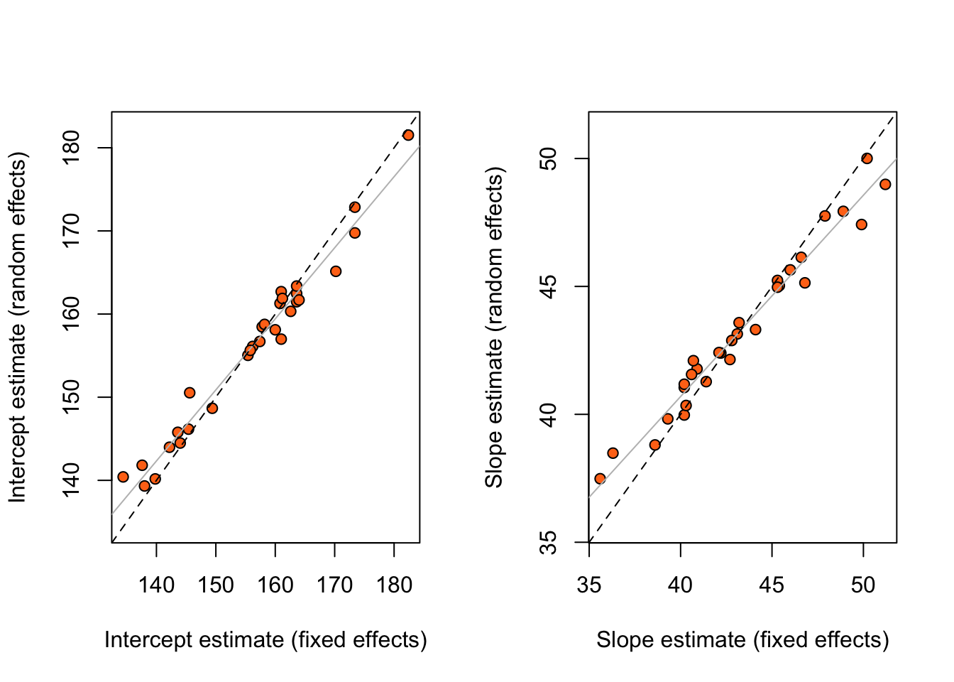
Figure Figure 2.4 shows parameter estimates from the random effects model against those from the fixed effects model, illustrating the shrinkage of the random effect estimates towards a common mean. Random effects estimates ‘borrow strength’ across clusters, due to the common \(\Sigma_b^{-1}\) term in (2.12). The extent of borrowing strength is determined by cluster similarity.
Figure 2.4: Estimates of random and fixed effects for the rat growth data. The dashed line is a line with intercept zero and slope 1, and the solid line is from the least squares fit of the observed points.
Bayesian inference: the Gibbs sampler
Bayesian inference for LMMs (and their generalizations, which we will introduce later) proceeds using Markov Chain Monte Carlo (MCMC) methods, such as the Gibbs sampler, that have proved very effective in practice.
MCMC computation provides posterior summaries, by generating a dependent sample from the posterior distribution of interest. Then, any posterior expectation can be estimated by the corresponding Monte Carlo sample mean, densities can be estimated from samples, etc.
MCMC will be covered in detail in the Computer Intensive Statistics APTS module. Here we simply describe the (most basic) Gibbs sampler.
To generate from \(f(y_1, \ldots , y_n)\), where the components \(y_i\) are allowed to be multivariate, the Gibbs sampler starts from an arbitrary value of \(y\) and updates components, sequentially or otherwise, by generating from the conditional distributions \(f(y_i \mid
y_{\setminus i})\) where \(y_{\setminus i}\) are all the variables other than \(y_i\), set at their currently generated values.
Hence, to apply the Gibbs sampler, we require conditional distributions which are available for sampling.
For the linear mixed model \[
Y \mid X, Z, \beta, \Sigma, b \sim {\mathop{\mathrm{N}}}(\mu, \Sigma),\quad \mu=X\beta+Zb,\quad b \mid \Sigma_b \sim \mathop{\mathrm{N}}(0,\Sigma_b) \, ,
\] and prior densities \(\pi(\beta)\), \(\pi(\Sigma)\), \(\pi(\Sigma_b)\), we obtain the conditional posterior distributions \[
\begin{aligned}
f(\beta\mid y,\text{rest}) & \propto \phi(y-Zb \,;\,X\beta,V)\pi(\beta)\,, \\
f(b\mid y,\text{rest})&\propto \phi(y-X\beta \,;\,Zb,V)\phi(b \,;\,0,\Sigma_b)\,, \\
f(\Sigma\mid y,\text{rest})&\propto \phi(y-X\beta-Zb \,;\,0,V)\pi(\Sigma)\,, \\
f(\Sigma_b\mid y,\text{rest})&\propto \phi(b \,;\,0,\Sigma_b)\pi(\Sigma_b) \,,
\end{aligned}
\] where \(\phi(y\,;\,\mu,\Sigma)\) is the density of a \({\mathop{\mathrm{N}}}(\mu,\Sigma)\) random variable evaluated at \(y\).
We can exploit conditional conjugacy in the choices of \(\pi(\beta)\), \(\pi(\Sigma)\), \(\pi(\Sigma_b)\) making the conditionals above of known form and, hence, straightforward to sample from. The conditional independence \((\beta, \Sigma) \perp\!\!\!\perp\Sigma_b \mid b\) is also helpful in that direction.
2.5 Generalized linear mixed models
Model setup
Generalized linear mixed models (GLMMs) generalize LMMs to non-normal responses, similarly to how generalized linear models generalize normal linear models. A GLMM has \[
\begin{aligned}
Y_i \mid x_i, z_i, b & \stackrel{\text{ind}}{\sim}\mathop{\mathrm{EF}}(\mu_i,\sigma^2)\,,\\
\begin{bmatrix} g(\mu_1)\\\vdots \\ g(\mu_n) \end{bmatrix} & = X \beta + Zb \, ,\\
b & \sim {\mathop{\mathrm{N}}}(0,\Sigma_b)\,,
\end{aligned}
\tag{2.14}\] where \(\mathop{\mathrm{EF}}(\mu_i,\sigma^2)\) is an exponential family distribution with mean \(\mu_i\) and variance \(\sigma^2 V(\mu_i) / m_i\) for known \(m_i\). For many well-used distributions, like binomial and Poisson, \(\sigma^2=1\). For the shake of not complicating presentation, we shall assume that from here on.
The normality of the random effects \(b\) can be relaxed in many ways and to other distributions, but normal random effects usually provide adequate fits. Non-normal random effects distributions are beyond the scope of this module.
Example 2.6 A random-intercept GLMM for binary data in \(k\) clusters with \(n_1, \ldots , n_k\) observations per cluster, and a single explanatory variable \(x\) (e.g. the setting for the toxoplasmosis data at individual level) is \[
\begin{aligned}
Y_{ij} \mid x_{ij}, b_{i} & \stackrel{\text{ind}}{\sim}\mathop{\mathrm{Bernoulli}}(\mu_{ij}) \\
\log\frac{\mu_{ij}}{1-\mu_{ij}} & = \beta_1 + b_{i} + \beta_2 x_{ij} \\
b_{i} & \stackrel{\text{ind}}{\sim}{\mathop{\mathrm{N}}}(0,\sigma^2_b)
\end{aligned}
\tag{2.15}\] This model fits into the general GLMM framework in (3.1) with \[
Y = \begin{bmatrix}
Y_1 \\
\vdots \\
Y_k
\end{bmatrix}\,, \quad
Y_i = \begin{bmatrix}
Y_{i1} \\
\vdots \\
Y_{in_i}
\end{bmatrix} \, ,
\]\[
X = \begin{bmatrix}
X_1 \\
\cdots \\
X_k
\end{bmatrix}\,, \quad
X_i = \begin{bmatrix}
1 & x_{i1} \\
\vdots & \vdots \\
1 & x_{in_i}
\end{bmatrix}\,,
\]\[
Z = \begin{bmatrix}
Z_1 & 0 & \cdots & 0 \\
0 & Z_2 & \cdots & 0 \\
\vdots & \vdots & \ddots & \vdots \\
0 & 0 & \cdots & Z_k
\end{bmatrix}\,, \quad
Z_i = \begin{bmatrix}
1 \\
\vdots \\
1
\end{bmatrix}\,,
\]\[
\beta = \begin{bmatrix}
\beta_1 \\
\beta_2
\end{bmatrix}\,, \quad
b = \begin{bmatrix}
b_1 \\
\vdots \\
b_k
\end{bmatrix}\,, \quad
\Sigma_b = \sigma^2_b I_k \, ,
\] and \(g(\mu) = \log \{ \mu / (1 - \mu) \}\).
GLMM likelihood
The marginal distribution of \(Y\) in a GLMM does not usually have a convenient closed-form representation. \[
\begin{aligned}
f(y \mid X, Z \,;\,\beta,\Sigma_b) & = \int f(y \mid X, Z, b \,;\,\beta, \Sigma_b)f(b \,;\,\beta, \Sigma_b)db \\
&= \int f(y \mid X, Z, b \,;\,\beta)f(b \,;\,\Sigma_b)db\\
&= \int \prod_{i=1}^n f\left(y_i \mid X, Z, b \,;\,\beta)\right) f(b \,;\,\Sigma_b)db\,.
\end{aligned}
\tag{2.16}\]
For nested random effects structures, some simplification is possible. For example, for (2.15), \[
f(y \mid X, Z \,;\,\beta,\sigma^2_b)
= \prod_{i=1}^k \int \prod_j f \left(y_{ij} \mid x_i, b_i \,;\,\beta)\right) \phi(b_i \,;\,0, \sigma^2_b)db_i \,,
\] which is a product of one-dimensional integrals.
Fitting a GLMM by likelihood methods requires some method for approximating the integrals involved.
When the integrals are of low dimension, a reliable method is to use Gaussian quadrature (see APTS: Statistical Computing). For example, for an one-dimensional cluster-level random effect \(b_i\) we might use \[
\begin{aligned}
& \int \prod_j f \left(y_{ij} \mid x_i, b_i \,;\,\beta)\right) \phi(b_i \,;\,0, \sigma^2_b)db_i \\
\approx & \sum_{q = 1}^Q W_q \prod_j f \left(y_{ij} \mid x_i, \sqrt{2} \sigma_b B_q \,;\,\beta)\right) / \sqrt{\pi}\, ,
\end{aligned}
\] for weights \(W_q\) and quadrature points \(B_q\)\((q = 1,\ldots ,Q)\) chosen according to the Gauss-Hermite quadrature rule.
Effective quadrature approaches use information about the mode and dispersion of the integrand, which can be done adaptively. For multi-dimensional \(b_i\), quadrature rules can be applied recursively, but performance in fixed-time diminishes rapidly with dimension.
An alternative approach is to use a Laplace approximation to the likelihood. Writing \[
h(b) = \prod_{i=1}^n f\left(y_i \mid X, Z, b \,;\,\beta\right) f(b \,;\,\Sigma_b)
\] for the integrand of the likelihood, a first-order Laplace approximation approximates \(h(.)\) as an unnormalised multivariate normal density function \[
\tilde h(b) = c \, \phi_k(b \,;\,\hat b, Q)\,,
\] where \(\hat b\) is found by maximizing \(\log h(.)\) over \(b\), the variance matrix \(Q\) is chosen so that the curvature of \(\log h(.)\) and \(\log \tilde h(.)\) agree at \(\hat b\), and \(c\) is chosen so that \(\tilde h(\hat b) = h(\hat b)\). The first-order Laplace approximation is equivalent to adaptive Gaussian quadrature with a single quadrature point.
Likelihood inference for GLMMs remains an area of active research and vigorous debate. Quadrature-based procedures provides accurate approximations to the likelihood. For some model structures, particularly those with crossed rather than nested random effects, the likelihood integral may be high-dimensional, and it may be impractical to use quadrature. In such cases, a Laplace approximation has been found to be sufficiently accurate for most purposes, but its accuracy is not guaranteed for every model.
Another alternative is to use Penalized Quasi Likelihood (PQL), which is very fast but often inaccurate. In, particular, PQL can fail badly in some cases, particularly with binary observations, and its use is not recommended.
Example 2.7 (Toxoplasmosis data (revisited)) For the toxoplasmosis data in Example 2.1, Table 2.1 gives the estimates and associated standard errors for the parameters of individual-level model (2.15), after dividing the annual rainfall by \(10^5\). The fits are obtained using maximum likelihood (with \(25\) quadrature points), Laplace approximation, and PQL.
Table 2.1: Estimates and associated standard errors for the parameters of the linear individual-level model (2.15). ‘GH (25)’ is maximum likelihood using \(25\) Gauss-Hermite quadrature points, ‘Laplace’ is maximum approximate likelihood based on Laplace approximation, and ‘PQL’ is maximum PQL.
GH (25)
Laplace
PQL
\(\beta_1\)
-0.138
-0.134
-0.115
(1.446)
(1.441)
(1.445)
\(\beta_2\)
0.722
0.592
0.057
(74.859)
(74.618)
(74.922)
\(\sigma_b\)
0.521
0.513
0.495
Table 2.2 shows the estimates for the corresponding GLMM, when the conditional mean of the incidence in toxoplasmosis is associated with an orthogonal polynomial to rainfall (after division by \(10^5\)); see ?poly.
Table 2.2: Estimates and associated standard errors for the parameters of the cubic individual-level model. ‘GH (25)’ is maximum likelihood with \(25\) Gauss-Hermite quadrature points, ‘Laplace’ is maximum approximate likelihood based on Laplace approximation, and ‘PQL’ is maximum PQL.
GH (25)
Laplace
PQL
\(\beta_1\)
-0.106
-0.104
-0.110
(0.127)
(0.126)
(0.127)
\(\beta_2\)
-0.106
-0.107
-0.098
(0.687)
(0.682)
(0.718)
\(\beta_3\)
0.154
0.149
0.173
(0.700)
(0.695)
(0.724)
\(\beta_4\)
1.628
1.626
1.607
(0.654)
(0.649)
(0.682)
\(\sigma_b\)
0.423
0.417
0.431
There is a good agreement between the different estimation methods for the models considered in this example. The AIC and BIC (using \(25\) Gauss-Hermite quadrature points for the likelihood approximation) for the linear and the cubic individual-level models are
As for LMMs, Bayesian inference in GLMMs is typically based on the Gibbs sampler. For the GLMM in (3.1), with prior densities \(\pi(\beta)\) and \(\pi(\Sigma_b)\) and known \(\sigma^2\), we obtain the conditional posterior distributions \[
\begin{aligned}
f(\beta\mid y,\text{rest}) & \propto \pi(\beta) \prod_i f(y_i \mid X, Z, \beta, b)\\
f(b\mid y,\text{rest}) & \propto \phi(b \,;\,0, \Sigma_b)\prod_i f(y_i \mid X, Z, \beta, b)\\
f(\Sigma_b \mid y, \text{rest}) & \propto \phi(b \,;\,0, \Sigma_b) \pi(\Sigma_b) \,,
\end{aligned}
\] For a conditionally conjugate choice of \(\pi(\Sigma_b)\), \(f(\Sigma_b
\mid y,\text{rest})\) is straightforward to sample from. The conditionals for \(\beta\) and \(b\) are not generally available for direct sampling. However, there are a number of ways of modifying the basic Gibbs sampling to go around this.
Akaike, H. (1973). Information theory and an extension of the maximum likelihood principle. In B. N. Petrov & F. Czáki (Eds.), Second international symposium on information theory (pp. 267–281). Akademiai Kiadó. https://doi.org/10.1007/978-1-4612-0919-5_38
Albert, J. H., & Chib, S. (1993). Bayesian analysis of binary and polychotomous response data. Journal of the American Statistical Association, 88, 669–679. https://doi.org/10.2307/2290350
Best, N., & Thomas, A. (2000). Bayesian graphical models and software for GLMs. In D. K. Dey, S. K. Ghosh, & B. K. Mallick (Eds.), Generalized linear models: A Bayesian perspective (pp. 387–406). Marcel Dekker. https://doi.org/10.1201/9781482293456
Breslow, N. E., & Clayton, D. G. (1993). Appproximate inference in generalised linear mixed models. Journal of the American Statistical Association, 88, 9–25. https://doi.org/10.2307/2290687
Burnham, K. P., & Anderson, D. R. (2002). Model selection and multi-model inference: A practical information theoretic approach (Second). Springer. https://doi.org/10.1007/978-1-4757-2917-7
Candès, E., & Tao, T. (2007). The Dantzig selector: Statistical estimation when \(p\) is much larger than \(n\) (with discussion). Annals of Statistics, 35, 2313–2404. https://doi.org/10.1214/009053606000001523
Cowell, R. G., Dawid, A. P., Lauritzen, S. L., & Spiegelhelter, D. J. (1999). Probabilistic networks and expert systems. Springer-Verlag. https://doi.org/10.1007/b97670
Dempster, A. P., Laird, N. M., & Rubin, D. B. (1977). Maximum likelihood from incomplete data via the EM algorithm (with discussion). Journal of the Royal Statistical Society Series B, 39, 1–38. https://doi.org/10.1111/j.2517-6161.1977.tb01600.x
Efron, B. (1975). Defining the curvature of a statistical problem (with applications to second order efficiency). The Annals of Statistics, 3(6), 1189–1242. https://doi.org/10.1214/aos/1176343282
Fan, J., & Li, R. (2001). Variable selection via nonconcave penalized likelihood and its oracle properties. Journal of the American Statistical Association, 96, 1348–1360.
Fan, J., & Lv, J. (2008). Sure independence screening for ultrahigh dimensional feature space (with Discussion). Journal of the Royal Statistical Society Series B, 70, 849–911. https://doi.org/10.1198/016214501753382273
Gelman, A., Carlin, J. B., Stern, H. S., Dunson, D. B., Vehtari, A., & Rubin, D. B. (2004). Bayesian data analysis (3rd ed.). Chapman; Hall/CRC. https://doi.org/10.1201/b16018
Gilks, W. R., Richardson, S., & Spiegelhalter, D. J. (Eds.). (1996). Markov chain monte carlo in practice. Chapman & Hall.
Green, P. J., Hjørt, N. L., & Richardson, S. (Eds.). (2003). Highly structured stochastic systems. Chapman & Hall/CRC. 10.1201/b14835
Hastie, T., Tibshirani, R., & Wainwright, M. (2015). Statistical learning with sparsity: The Lasso and generalizations. Chapman; Hall/CRC. https://doi.org/10.1201/b18401
Hoeting, J. A., Madigan, D., Raftery, A. E., & Volinsky, C. T. (1999). Bayesian model averaging: A tutorial (with discussion). Statistical Science, 14, 382–417. https://doi.org/10.1214/ss/1009212519
Jamshidian, M., & Jennrich, R. I. (1997). Acceleration of the EM algorithm by using quasi-Newton methods. Journal of the Royal Statistical Society Series B, 59, 569–587. https://doi.org/10.1111/1467-9868.00083
Liang, K., & Zeger, S. L. (1986). Longitudinal data analysis using generalized linear models. Biometrika, 73(1), 13–22. https://doi.org/10.1093/biomet/73.1.13
Marin, J.-M., & Robert, C. P. (2007). Bayesian core: A practical approach to computational bayesian statistics. Springer-Verlag. https://doi.org/10.1007/978-0-387-38983-7
McQuarrie, A. D. R., & Tsai, C.-L. (1998). Regression and time series model selection. World Scientific. https://doi.org/10.1142/3573
Meng, X.-L., & van Dyk, D. (1997). The EM algorithm — an old folk-song sung to a fast new tune (with discussion). Journal of the Royal Statistical Society Series B, 59, 511–567. https://doi.org/10.1111/1467-9868.00082
Nelder, J. A., Lee, Y., & Pawitan, Y. (2017). Generalized linear models with random effects: A unified approach via \(h\)-likelihood (2nd ed.). Chapman; Hall/CRC. https://doi.org/10.1201/9781315119953
Nelder, J. A., & Wedderburn, R. W. M. (1972). Generalized linear models. Journal of the Royal Statistical Society: Series A (General), 135(3), 370–384. https://doi.org/10.2307/2344614
Oakes, D. (1999). Direct calculation of the information matrix via the EM algorithm. Journal of the Royal Statistical Society Series B, 61, 479–482. https://doi.org/10.1111/1467-9868.00188
Ogden, H. (2021). On the error in laplace approximations of high-dimensional integrals. Stat, 10(1), e380. https://doi.org/10.1002/sta4.380
Ogden, H. E. (2017). On asymptotic validity of naive inference with an approximate likelihood. Biometrika, 104(1), 153–164. https://doi.org/10.1093/biomet/asx002
Pinheiro, J., & Bates, D. M. (2002). Mixed effects models in S and S-PLUS. New York:Springer-Verlag. https://doi.org/10.1007/b98882
Raftery, A. E., Madigan, D., & Hoeting, J. A. (1997). Bayesian model averaging for linear regression models. Journal of the American Statistical Association, 92, 179–191. https://doi.org/10.1080/01621459.1997.10473615
Richardson, S., & Green, P. J. (1997). On bayesian analysis of mixtures with an unknown number of components (with discussion). Journal of the Royal Statistical Society Series B, 59, 731–792. https://doi.org/10.1111/1467-9868.00095
Spiegelhalter, D. J., Best, N. G., Carlin, B. P., & Linde, A. van der. (2002). Bayesian measures of model complexity and fit (with discussion). Journal of the Royal Statistical Society, Series B, 64, 583–639. https://doi.org/10.1111/1467-9868.00353
Tanner, M. A. (1996). Tools for statistical inference: Methods for the exploration of posterior distributions and likelihood functions (Third). Springer. https://doi.org/10.1007/978-1-4612-4024-2
Wedderburn, R. W. M. (1974). Quasi-Likelihood Functions, Generalized Linear Models, and the Gauss-Newton Method. Biometrika, 61(3), 439. https://doi.org/10.2307/2334725