Remember that all models are wrong; the practical question is how wrong do they have to be to not be useful.
— George Box (1919 – 2013)
in Box and Draper (1987). Empirical Model-Building and Response Surfaces, p. 74
1.1 Introduction
Statisticians construct models to simplify reality, to gain understanding, to compare scientific, economic, or other theories, and to predict future events or data. We rarely believe in our models, but regard them as temporary constructs, which should be subject to improvement. Often we have several models and must decide which, if any, is preferable.
Principles for model selection include:
Substantive knowledge, from previous studies, theoretical arguments, dimensional or other general considerations.
Robustness to departures from assumptions: we prefer models that provide valid inference even if some of their assumptions are invalid.
Quality of fit: we prefer models that perform well in terms of informal devices such as residuals and graphical assessments, or more formal or goodness-of-fit tests.
Parsimony: for reasons of economy we seek the simplest possible models that are adequate descriptions of the data.
There may be a very large number of plausible models for us to compare. For instance, in a linear regression with \(p\) covariates, there are \(2^p\) possible combinations of covariates: for each covariate, we need to decide whether or not to include that variable in the model. If \(p = 20\) we have over a million possible models to consider, and the problem becomes even more complex if we allow for transformations and interactions in the model.
To focus and simplify discussion we will consider model selection among parametric models, but the ideas generalize to semi-parametric and non-parametric settings.
Example 1.1 (Nodal involvement data) A logistic regression model for binary responses assumes that \(Y_i \mid x_i \sim \mathop{\mathrm{Bernoulli}}(\mu_i)\), with \(\mu_i = P(Y_i = 1 \mid x_i)\), and a linear model for log odds \[
\log\left(\frac{\mu_i}{1-\mu_i}\right) = x_i^\top \beta \, .
\] The log-likelihood about \(\beta\), assuming that \(Y_1, \ldots, Y_n\) are independent conditionally on the covariate vectors \(x_1, \ldots, x_n\), is \[
\ell(\beta) = \sum_{i=1}^n y_i x_i^\top \beta - \sum_{i=1}^n \log\left\{1 + \exp( x_i^\top \beta)\right\} \, .
\] A good fit gives large maximized log-likelihood \(\hat
\ell = \ell(\hat\beta)\) where \(\hat\beta\) is the maximum likelihood estimator.
The SMPracticals R package contains a dataset called nodal, which relates to the nodal involvement (r) of 53 patients with prostate cancer, with five binary covariates aged, stage, grade, xray and acid.
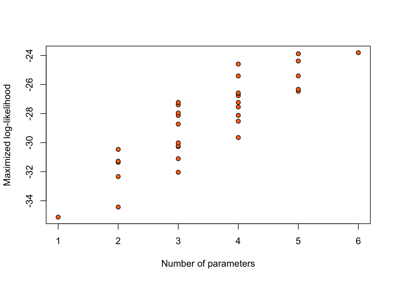
Considering only the models without any interaction between the 5 binary covariates, results in \(2^5 = 32\) possible logistic regression models for this data. We can rank these models according to the value of the maximized log-likelihood \(\hat \ell\). Figure 1.1 summarizes such a ranking through a plot of the maximized log-likelihood of each of the 32 models under consideration against the number of unknown parameters in each model.
Figure 1.1: Maximized log-likelihoods for 32 possible logistic regression models for the nodal data.
Adding terms always increases the maximized log-likelihood \(\hat\ell\). So, taking the model with highest \(\hat\ell\) would give the full model. We need to a different way to compare models, which should trade off quality of fit (measured by \(\hat \ell\)) and model complexity (number of parameters or, more generally, degrees of freedom).
1.2 Criteria for model selection
Likelihood inference under the wrong model
Suppose the (unknown) true model has independent \(Y_1, \ldots, Y_n\), where \(Y_i\) has a density or probability mass function \(g(y)\). Suppose we have a candidate model that assumes \(Y_1, \ldots, Y_n\) are independent where \(Y_i\) has a density of probability mass function \(f(y \,;\,\theta)\). We wish to compare the candidate model against other candidate models. For each candidate model, we first find the maximum likelihood estimate \(\hat \theta\) of the model parameters, and, then, use criteria based on the maximized log-likelihood \(\hat \ell = \ell(\hat \theta)\) to compare candidate models.
We do not assume that any of the candidate models are correct; there may be no value of \(\theta\) such that \(f(\cdot \,;\,\theta) = g(\cdot)\). Before we can decide on an appropriate criterion for choosing between models, we first need to understand the asymptotic behaviour of \(\hat \theta\) and \(\ell(\hat \theta)\) without the usual assumption that the model is correctly specified.
The log-likelihood \(\ell(\theta)\) of the candidate model is maximized at \(\hat\theta\), and \[
\bar \ell(\hat\theta) = n^{-1}\ell(\hat\theta) \to \int \log f(y \,;\,\theta_g) g(y)\, dy,\quad \text{almost surely as } n\to\infty \,,
\] where \(\theta_g\) minimizes the Kullback-Leibler divergence \[
KL(f_\theta,g) =
\int \log\left\{ \frac{g(y)}{f(y \,;\,\theta)}\right\} g(y) \, dy \,.
\]
Theorem 1.1 Suppose the true model has \(Y_1, \ldots, Y_n\) independent with \(Y_i\) having a density or probability mass function \(g(y)\), but, instead, we assume that \(Y_i\) has a density or probability mass function \(f(y \,;\,
\theta)\). Then under mild regularity conditions, the maximum likelihood estimator \(\hat\theta\) satisfies \[
\sqrt{n} (\hat\theta - \theta_g) \stackrel{d}{\rightarrow} {\mathop{\mathrm{N}}}\left( 0,
n I(\theta_g)^{-1}K(\theta_g)I(\theta_g)^{-1}\right) \,,
\tag{1.1}\] where \[
\begin{aligned}
K(\theta) &= n \int
\frac{\partial \log f(y \,;\,\theta)}{\partial\theta} \frac{\partial \log
f(y \,;\,\theta)}{\partial\theta^\top }g(y)\, dy,\\ I(\theta) &= -n \int
\frac{\partial^2 \log f(y \,;\,\theta)}{\partial\theta\partial\theta^\top }
g(y)\, dy \, .
\end{aligned}
\] The likelihood ratio statistic converges in distribution as \[
W(\theta_g) = 2\left\{\ell(\hat\theta)-\ell(\theta_g)\right\} \stackrel{d}{\rightarrow}
\sum_{r=1}^p \lambda_r V_r \,,
\] where \(V_1, \ldots, V_p\) are independent with \(V_i \sim \chi^2_1\), and \(\lambda_r\) are eigenvalues of \(K(\theta_g)^{1/2}I(\theta_g)^{-1}
K(\theta_g)^{1/2}\). Thus, \(E\{W(\theta_g)\} \rightarrow \mathop{\mathrm{tr}}\{I(\theta_g)^{-1}K(\theta_g)\}\).
Under the true model, \(\theta_g\) is the ‘true’ value of \(\theta\), \(K(\theta) = I(\theta)\), \(\lambda_1 = \cdots = \lambda_p = 1\), and we recover the usual results.
In practice \(g(y)\) is, of course, unknown, and then \(K(\theta_g)\) and \(I(\theta_g)\) may be estimated by \[
\hat K = \sum_{i=1}^n \frac{\partial \log f(y_i \,;\,\hat\theta)}{\partial\theta}
\frac{\partial \log f(y_i \,;\,\hat\theta)}{\partial\theta^\top }, \quad
\hat J = - \sum_{i=1}^n \frac{\partial^2 \log f(y_i \,;\,\hat\theta)}
{\partial\theta\partial\theta^\top } \, .
\]
The latter is just the observed information matrix. We can then construct confidence regions and hypothesis tests about \(\theta_g\), using the fact that, from (1.1), the approximate distribution of \(\hat\theta\) is \({\mathop{\mathrm{N}}}\left( \theta_g,
I(\theta_g)^{-1}K(\theta_g)I(\theta_g)^{-1}\right)\) and replacing the variance covariance matrix with \(\hat J^{-1}\hat K\hat J^{-1}\).
Information criteria
Using the average log-likelihood \(\bar \ell(\hat \theta)\) to choose between models leads to overfitting, because we use the data twice: first to estimate \(\theta\), then again to evaluate the model fit.
If we had another independent sample \(Y_1^+,\ldots,Y_n^+\sim g\) and computed \[
\bar\ell^+(\hat\theta) = n^{-1}\sum_{i=1}^n \log f(Y^+_i \,;\,\hat\theta)\,,
\] we would choose choose the candidate model that maximizes \[
\Delta = {\mathop{\mathrm{E}}}_g\left[ {\mathop{\mathrm{E}}}^+_g\left\{ \bar\ell^+(\hat\theta) \right\} \right] \,,
\tag{1.2}\] where the inner expectation is over the distribution of \(Y_i^+\), and the outer expectation is over the distribution of \(\hat\theta\).
Since \(g(.)\) is unknown, we cannot compute \(\Delta\) directly. We will show that \(\bar \ell(\hat \theta)\) is a biased estimator of \(\Delta\), but by adding an appropriate penalty term we can obtain an approximately unbiased estimator of \(\Delta\), which we can use for model comparison.
We write \[
{\mathop{\mathrm{E}}}_g\{\bar \ell(\hat \theta)\} =
\underbrace{{\mathop{\mathrm{E}}}_g\{\bar \ell(\hat \theta) - \bar \ell(\theta_g)\}}_{a}
+ \underbrace{{\mathop{\mathrm{E}}}_g\{\bar \ell(\theta_g)\} - \Delta}_{b}
+ \Delta \, .
\] Then, \(a + b\) is the bias in using \(\bar \ell(\hat \theta)\) to estimate \(\Delta\). Hence, finding expressions for \(a\) and \(b\) would allow us to correct for that bias. We have \[
a = {\mathop{\mathrm{E}}}_g\{\bar\ell(\hat\theta) - \bar\ell(\theta_g)\}
= \frac{1}{2n}E_g\{W(\theta_g)\}
\approx \frac{1}{2n}\mathop{\mathrm{tr}}\{I(\theta_g)^{-1} K(\theta_g)\} \,.
\] Results on inference under the wrong model (we will not prove this here) may be used to show that \[
b = {\mathop{\mathrm{E}}}_g\{\bar \ell(\theta_g)\} - \Delta \approx \frac{1}{2n}
\mathop{\mathrm{tr}}\{I(\theta_g)^{-1} K(\theta_g)\} \, .
\] Putting the latter two expressions together, we have \[
{\mathop{\mathrm{E}}}_g\{\bar \ell(\hat \theta)\} = \Delta + a + b = \Delta + \frac{1}{n}
\mathop{\mathrm{tr}}\{I(\theta_g)^{-1} K(\theta_g)\} \,.
\]
So, in order to correct the bias in using \(\bar\ell(\hat\theta)\) to estimate \(\Delta\), we can aim to maximize \[
\bar\ell(\hat\theta) - \frac{1}{n}\mathop{\mathrm{tr}}(\hat J^{-1} \hat K) \, ,
\] over the candidate models. Equivalently, we can maximize \[
\hat \ell - \mathop{\mathrm{tr}}(\hat J^{-1} \hat K) \,,
\] or, equivalently, minimize \[
2\{\mathop{\mathrm{tr}}(\hat J^{-1}\hat K)-\hat\ell\} \,,
\] The latter expression is called the Takeuchi Information Criterion and has also been refereed to as the Network Information Criterion.
Let \(p = \dim(\theta)\) be the number of parameters in a candidate model, and \(\hat\ell\) the corresponding maximized log likelihood. There are many other information criteria with a variety of penalty terms:
Name
Acronym
Criterion
Akaike Information Criterion
AIC
\(2(p - \hat\ell)\)
Corrected AIC
AIC\(_\text{c}\)
\(2(p + (p^2 + p) / (n - p - 1) - \hat\ell)\)
Bayesian Information Criterion
BIC
\(2(p \log n / 2 - \hat\ell)\)
Deviance Information Criterion
DIC
Extended Information Criterion
EIC
Generalized Information Criterion
GIC
\(\vdots\)
Another popular model selection criterion for regression problems is Mallows’ \(C_p = \text{RSS}/s^2 + 2p-n\), where \(\text{RSS}\) is the residual sum of squares of the candidate model, and \(s^2\) is an estimate of the error variance \(\sigma^2\).
Example 1.2 (Nodal involvement data (revisited)) AIC and BIC can both be used to choose between the \(2^5\) models that we fitted to the nodal involvement data in Example 1.1.
Both criteria prefer a model with four parameters, which includes three of the five covariates: acid, stage and xray.
Figure 1.2 shows the AIC and BIC for each of the \(32\) models, against the number of free parameters. As is apparent, BIC increases more rapidly than AIC after the minimum, as it penalizes more strongly against model complexity, as measured by the number of free parameters.
Code
par(mfrow =c(1, 2))plot(AIC ~ df, data = mods_AIC, xlab ="Number of parameters",bg ="#ff7518", pch =21)plot(BIC ~ df, data = mods_BIC, xlab ="Number of parameters",bg ="#ff7518", pch =21)
Figure 1.2: AIC and BIC for 32 logistic regression models for the nodal data.
Theoretical properties of information criteria
We may assume that the true model is of infinite dimension, and that by choosing among our candidate models we hope to get as close as possible to this ideal model, using the available data. We need some measure of distance between a candidate and the true model, and we aim to minimize that distance. A model selection procedure that selects the candidate closest to the truth for large \(n\) is called asymptotically efficient.
An alternative is to suppose that the true model is among the candidate models. If so, then a model selection procedure that selects the true model with probability tending to one as \(n\to\infty\) is called consistent.
We seek to find the correct model by minimizing and information criterion \(\text{IC} = c(n,p) - 2\hat\ell\), where the penalty \(c(n,p)\) depends on sample size \(n\) and the dimension \(p\) of the parameter space.
A crucial aspect in the behaviour of model selection procedures is the differences in IC. Let IC be an information criterion for the true model, and IC\(_+\) an information criterion for a model with one extra parameter.
Table 1.1 lists the value of \(c(n,p+1) - c(n,p)\) for AIC, TIC, and BIC.
Table 1.1: Difference in IC penalties
Criterion
\(c(n,p+1) - c(n,p)\)
AIC
\(= 2\)
TIC
\(\approx 2\) for large \(n\)
BIC
\(= \log n\)
Under regularity conditions about the model and as \(n \to \infty\), \(2(\hat\ell_+-\hat\ell)\) converges in distribution to a \(\chi^2_1\) random variable. So, as \(n\to\infty\), \[
P(\text{IC}_+<\text{IC}) \to
\begin{cases}
0.157, & \text{if AIC or TIC is used} \\
0, & \text{if BIC is used}
\end{cases} \, .
\] Thus, in contrast to BIC, AIC and TIC have non-zero probability of selecting a model with an extra parameter (over-fitting), even in very large samples.
1.3 Variable selection for linear models
Consider a linear regression model \[
Y = X^*\beta + \epsilon\,,
\] with \(\mathop{\mathrm{E}}(\epsilon) = 0\) and \(\mathop{\mathrm{cov}}(\epsilon) = \sigma^2 I_n\), where \(X^*\) is an \(n \times p^*\) model matrix with columns \(v_j\), for \(j \in
\mathcal{I}= \{1, \ldots, p^*\}\), \(Y = (Y_1, \ldots, Y_n)^\top\), and \(\beta =
(\beta_1, \ldots, \beta_{p^*})^\top\) is the vector of regression parameters.
Assume that the data generating process is a linear regression model of \(Y\) on a subset \(\mathcal{J}\subseteq \mathcal{I}\) of the columns of \(X^*\) with \(|\mathcal{J}| = p_0 \le p^*\), and the goal is to estimate \(\mathcal{J}\) based on data.
The parameters \(\beta\) enter the model through a linear predictor. So, selecting columns of \(X^*\) is formally equivalent to estimating the sets \[
\mathcal{J}= \{j \in \mathcal{I}: \beta_j \ne 0\} \quad
\text{and} \quad \mathcal{K}= \{j \in \mathcal{I}: \beta_j = 0\} \, ,
\] indicating which covariates should and should not be in the model, respectively.
A selected model can be either true, correct, or wrong. A true model has only those columns of $X^* with indices in \(\mathcal{J}\). A correct model has the columns of $X^* with indices in \(\mathcal{S}\), where \(\mathcal{J}\subseteq \mathcal{S}\subseteq \mathcal{I}\). A wrong model has the columns of $X^* with indices \(\mathcal{S}\), where \(\mathcal{S}\not\subset \mathcal{J}\).
Suppose we fit a candidate model \(Y = X\beta + \epsilon\), with \(X\) having the columns of \(X^*\) with indices in \(\mathcal{S}\subseteq \mathcal{I}\) with \(|\mathcal{S}| = p \le p^*\). The fitted values are \[
X\hat\beta = X \{ (X^\top X)^{-1}X^\top Y\} = H Y = H\mu + H \epsilon\,,
\] where \(\mu = X^* \beta\) is the expectation of \(Y\), and \(H = X (X^\top
X)^{-1} X^\top\) is the hat matrix. It is a simple exercise to show that \(H \mu = \mu\) if the model is correct.
As with AIC, suppose we have an independent set of responses \(Y_+\) with \(Y_+ = \mu + \epsilon_+\), where \(\epsilon_+\) and \(\epsilon\) are independent, and \(\mathop{\mathrm{E}}(\epsilon_+) = 0\) and \(\mathop{\mathrm{cov}}(\epsilon_+) = \sigma^2 I_n\). A natural measure of prediction error in linear regression is the mean squared error \[
\Delta = n^{-1} {\mathop{\mathrm{E}}} \left[{\mathop{\mathrm{E}}}_+\left\{ (Y_+ - X\hat\beta)^\top (Y_+ - X\hat\beta) \right\}\right] \,,
\] where expectations are taken over both \(Y\) and \(Y_+\).
Theorem 1.2\[
\Delta =
\begin{cases}
n^{-1}\mu^\top (I_n - H)\mu + (1+p/n)\sigma^2\,, & \text{if the model is wrong}\\
(1+p/n)\sigma^2\,, & \text{if the model is correct} \\
(1+p_0/n)\sigma^2\,, & \text{if the model is true}\\
\end{cases} \, .
\tag{1.3}\]
Proof. We have \[
Y_{+} - X\hat\beta = Y_{+} - H Y = \mu + \epsilon_{+} - H \mu - H \epsilon = (I_n - H) \mu + (\epsilon_{+} - H \epsilon) \, .
\] Hence, \[
(Y_{+} - X\hat\beta)^\top (Y_{+} - X\hat\beta) = \mu (I_n - H) \mu + \epsilon_{+}^\top \epsilon_{+} + \epsilon^\top H \epsilon + Z \, ,
\] where \(Z\) collects all terms with \({\mathop{\mathrm{E}}}[{\mathop{\mathrm{E}}}_{+}(Z)] = 0\). From the assumptions on the errors, we have \({\mathop{\mathrm{E}}}[{\mathop{\mathrm{E}}}_{+}(\epsilon_{+}^\top
\epsilon_{+})] = n \sigma^2\), and \({\mathop{\mathrm{E}}}[{\mathop{\mathrm{E}}}_{+}(\epsilon^\top H
\epsilon)] = \mathop{\mathrm{tr}}{H}\sigma^2 = p\sigma^2\). Collecting terms, \[
\Delta = \underbrace{\mu (I_n - H) \mu / n}_{\text{Bias}} + \overbrace{(1 + p / n) \sigma^2}^\text{Variance} \, .
\] If the model is correct then \(H \mu = \mu\), and the bias term is zero. If the model is also true, then \(p = p_0\).
The bias term \(n^{-1}\mu^\top (I_n - H) \mu = n^{-1}\|\mu -
H\mu\|_2^2\) is positive, unless the model is correct, in which case it is zero. Its size is reduced the closer \(\mu\) is to the space spanned by the columns of \(X\) (or, equivalently, the closer \(\mu\) is to its projected value \(H \mu\)), and, hence we would expect a reduction in bias when useful covariates are added to the model. The variance term \((1 + p/n) \sigma^2\) increases as \(p\) increases, for example whenever useless terms are included. Ideally, we would choose a model matrix \(X\) to minimize \(\Delta\), but this is impossible, because \(\Delta\) depends on the unknowns \(\mu\) and \(\sigma\). We will have to estimate \(\Delta\).
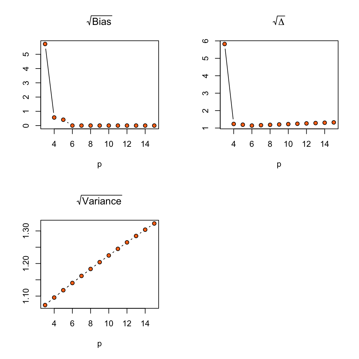
Example 1.3 (Polynomial regression) Consider the candidate models \[
Y_i = \sum_{j = 0}^{p - 1} \beta_j x_i^j + \epsilon_i \quad (i = 1, \ldots, n)\, ,
\] where \(x_1, \ldots, x_n\) have been generated from \(n\) independent standard normal random variables. Assume that the true model is \(Y_i
= \sum_{j = 0}^{5} x_i^j + \epsilon_i\), hence \(\mu_i = \sum_{j = 0}^{5}
x_i^j\) is a degree five polynomial, so \(p_0 = 6\).
Let \(n = 20\), and \(\sigma^2 = 1\). Figure 1.3 shows \(\sqrt{\Delta}\) for models of increasing polynomial degree, from the intercept only model (\(p = 1\)), to a linear model (\(p = 2\)), to a quadratic model (\(p = 3\)), up to a degree 14 polynomial (\(p = 15\)). The minimum of \(\Delta\) is achieved at \(p = p_0 = 6\). There is a sharp decrease in bias as useful covariates are added, and a slow increase with variance as the number of variables \(p\) increases.
Code
Delta <-function(p, p0, x, sigma2) { cols <-0:(p -1) cols0 <-0:(p0 -1) n <-length(x) X <-matrix(rep(x, p)^rep(cols, each = n), nrow = n) X0 <-matrix(rep(x, p0)^rep(cols0, each = n), nrow = n) mu <-rowSums(X0) H <-tcrossprod(qr.Q(qr(X))) bias <-sum(((diag(n) - H) %*% mu)^2) / n variance <- sigma2 * (1+ p / n)c(p = p, bias = bias, variance = variance)}n <-20sigma2 <-1p_max <-15set.seed(1)x <-rnorm(n)D <-data.frame(t(sapply(1:p_max, Delta, p0 =6, x = x, sigma2 =1)))par(mfrow =c(2, 2))plot(sqrt(bias) ~ p, data = D, subset = p >2,main =expression(sqrt("Bias")), ylab ="",type ="b", bg ="#ff7518", pch =21)plot(sqrt(bias + variance) ~ p, data = D, subset = p >2,main =expression(sqrt(Delta)), ylab ="",type ="b", bg ="#ff7518", pch =21)plot(sqrt(variance) ~ p, data = D, subset = p >2,main =expression(sqrt("Variance")), ylab ="", type ="b", bg ="#ff7518", pch =21)
Figure 1.3: \(\Delta\) for models with varying polynomial degree.
One approach to estimate \(\Delta\) is to split the data into two parts, \((X, y)\) and \((X_{+}, y_{+})\), where \(X_{+}\) is an \(n_{+} \times p\) matrix and \(y_{+}\) is the vector of the corresponding \(n_{+}\) response values. Then, we use the former part to estimate the candidate models, and the latter part to compute the prediction error. We compute \[
\hat\Delta = \frac{1}{n_{+}}(y_{+} -
X_{+}\hat\beta)^\top (y_{+} - X_{+}\hat\beta) = \frac{1}{n_{+}}\sum_{i = 1}^{n_{+}}(y_{+, i} - x_{+, i}^\top \hat\beta)^2\,,
\] where \(\hat\beta\) is the least squares estimator of the candidate model.
The available data may be either small for splitting, and, more generally, data splitting is not the most efficient use of the available information. For this reason, we often use leave-one-out cross-validation to estimate \(\Delta\) as \[
\hat\Delta_\text{CV} = \frac{1}{n} \sum_{i=1}^n (y_i - x_i^\top \hat\beta_{-i})^2 \,,
\tag{1.4}\] where \(\hat\beta_{-j}\) is the estimate computed without the \(i\)th observation. At first glance, (1.4) seems to require \(n\) fits of model. However, it can be shown that \[
\hat\Delta_\text{CV} = \frac{1}{n} \sum_{i=1}^n \frac{(y_i - x_i^\top \hat\beta)^2}{(1 - h_{ii})^2}\,,
\] where \(h_{11},\ldots, h_{nn}\) are diagonal elements of \(H\). So, (1.4) can be obtained from one fit.
A simpler, and often more stable, estimator than \(\hat\Delta_\text{CV}\) uses generalized cross-validation and has the form \[
\hat\Delta_\text{GCV} = \frac{1}{n} \sum_{i = 1}^n \frac{(y_i - x_i^\top \hat\beta)^2}{\{1 - \mathop{\mathrm{tr}}(H)/n\}^2}\,.
\]
Theorem 1.3\[
\mathop{\mathrm{E}}(\hat \Delta_\text{GCV}) = \frac{1}{n(1 - p / n)^2} \mu^\top (I_n - H)\mu + \frac{1}{1 - p / n} \sigma^2 \, .
\] Furthermore, for large \(n\), \(\mathop{\mathrm{E}}(\hat \Delta_\text{GCV}) \approx \Delta\), with \(\Delta\) as in (1.3).
Proof. It holds that \(Y - X\hat\beta = (I_n - H) Y = (I_n - H) \mu + (I_n - H) \epsilon\). So, \[
(Y - X\hat\beta)^\top (Y - X\hat\beta) = \mu^\top (I_n - H) \mu + \epsilon^\top (I_n - H) \epsilon + Z \,,
\] where the terms collected in \(Z\) have expectation zero. Using the fact that \(\mathop{\mathrm{tr}}{H} = p\), \[
\begin{aligned}
\mathop{\mathrm{E}}(\hat \Delta_\text{GCV}) & = \frac{1}{n(1 - p / n)^2}\mu^\top (I_n - H) \mu + \frac{(n - p)}{n(1 - p / n)^2} \sigma^2 \\
& = \frac{1}{n(1 - p / n)^2} \mu^\top (I_n - H) \mu + \frac{1}{1 - p/n}\sigma^2 \, .
\end{aligned}
\tag{1.5}\] For large \(n\) or small \(z = 1 / n\), a Taylor expansion of \((1 - p z)^{-1}\) about \(z = 0\) gives \((1 - p z)^{-1} = 1 + p z + O(z^2)\). Also, \(z (1 - z p)^{-2} = z + O(z^2)\). Replacing \((1 - p/n)^{-1}\) and \(n^{-1}(1 - p / n)^{-2}\) in the last expression in (1.5) with their first order approximations gives the right hand side of (1.3).
We can minimize either \(\hat\Delta_\text{CV}\) or \(\hat\Delta_\text{GCV}\). Model selection based on leave-one-out cross validation has been found to be less stable than generalized cross-validation. Another estimator of \(\Delta\) is obtained using \(k\)-fold cross-validation. \(k\)-fold cross-validation operates by splitting the data into \(k\) roughly equal parts (say \(k = 10\)), predicting the response for each part based on the model fit from the other \(k - 1\) parts, and, then, selecting the model that minimizes an aggregate estimate of prediction error.
1.4 A Bayesian perspective on model selection
In a parametric model, the data \(y\) is assumed to be a realization of \(Y\) with density or probability mass function \(f(y \mid \theta)\), where \(\theta\in\Omega_\theta\).
Separate from data, the prior information about the parameter \(\theta\) is summarized in a prior density or probability mass function \(\pi(\theta)\). The posterior density for \(\theta\) is given by Bayes’ theorem as \[
\pi(\theta\mid y ) = \frac{\pi(\theta) f(y\mid\theta)}{\int \pi(\theta) f(y\mid\theta)\, d\theta}\,.
\] Here \(\pi(\theta \mid y)\) contains all information about \(\theta\), conditional on the observed data \(y\). If \(\theta =
(\psi^\top,\lambda^\top)^\top\), then inference for \(\psi\) is based on the marginal posterior density or probability mass function\[
\pi(\psi\mid y) = \int \pi(\theta\mid y )\, d\lambda \,.
\]
Now, suppose we have \(M\) alternative models for the data, with respective parameters \(\theta_1 \in \Omega_{\theta_1}, \ldots,
\theta_M \in \Omega_{\theta_M}\). The spaces \(\Omega_{\theta_m}\) may have different dimensions.
We enlarge the parameter space to define an encompassing model with parameter \[
\theta \in \Omega = \bigcup_{m=1}^M \{m\}\times \Omega_{\theta_m}\,.
\] We need priors \(\pi_m(\theta_m\mid m)\) for the parameters of each model, plus a prior \(\pi(m)\) giving pre-data probabilities for each of the models. Then, for each model we have \[
\pi(m, \theta_m) = \pi(\theta_m\mid m)\pi(m) \, .
\]
Inference about model choice is based on the marginal posterior \[
\begin{aligned}
\pi(m\mid y) & = \frac{\int f(y\mid\theta_m)\pi_m(\theta_m)\pi(m)\, d\theta_m}
{\sum_{m'=1}^M \int f(y\mid\theta_{m'})\pi_{m'}(\theta_{m'})\pi(m')\, d\theta_{m'}} \\
& =
\frac{\pi(m) f(y\mid m)}
{\sum_{m'=1}^M \pi(m') f(y\mid{m'})}\,.
\end{aligned}
\tag{1.6}\]
For each model, we can write the joint posterior of model and parameters as \[
\pi(m, \theta_m \mid y) =\pi(\theta_m \mid m, y)\pi(m \mid y) \, ,
\] so Bayesian updating corresponds to the map \[
\pi(\theta_m\mid m)\pi(m) \mapsto \pi(\theta_m \mid m, y)\pi(m\mid y) \, .
\] So, for each model \(m \in \{1,\ldots, M\}\), it is necessary to compute
the posterior probability \(\pi(m\mid y)\), which involves the marginal likelihood \(f(y\mid m) = \int f(y\mid\theta_m,m)\pi(\theta_m\mid m)\, d\theta_m\); and
the posterior density \(\pi(\theta_m\mid y, m)\).
If there are just two models, we can write \[
\frac{\pi(1\mid y)}{\pi(2\mid y)} = \frac{\pi(1)}{\pi(2)} \frac{f(y\mid 1)}{f(y\mid 2)},
\] so the posterior odds on model 1 equal the prior odds on model 1 multiplied by the Bayes factor\(B_{12} = {f(y\mid 1)/ f(y\mid 2)}\).
Example 1.4 (Lindley’s paradox) Suppose the prior for each \(\theta_m\) is \(N(0, \sigma^2 I_{p_m})\), where \(p_m = \dim(\theta_m)\). Then, \[
\begin{aligned}
f(y \mid m) &= \sigma^{-p_m} (2\pi)^{-p_m/2} \int f(y \mid m, \theta_m) \prod_{r = 1}^{p_m} \exp \left\{-{\theta_{m,r}^2/(2\sigma^2)}\right\}
d\theta_{m, r}\\
& \approx \sigma^{-p_m} (2\pi)^{-p_m/2} \int f(y \mid m, \theta_m) \prod_{r = 1}^{p_m} d\theta_{m, r},
\end{aligned}
\] for a highly diffuse prior distribution (large \(\sigma^2\)). The Bayes factor for comparing the models is then approximately \[
\frac{f(y\mid 1)}{f(y\mid 2)}\approx \sigma^{p_2 - p_1} g(y),
\] where \(g(y)\) depends on the two likelihoods but is independent of \(\sigma^2\). Hence, whatever the data tell us about the relative merits of the two models, the Bayes factor in favour of the simpler model can be made arbitrarily large by increasing \(\sigma\). This illustrates Lindley’s paradox, and highlights that we must be careful when specifying prior dispersion parameters when comparing models.
If a quantity \(Z\) has the same interpretation for all models, it is desirable to allow for model uncertainty when constructing inferences or making predictions about it.
If prediction is the aim, the each model may be just a vehicle that provides a future value, and not of interest on its own.
If \(Z\) corresponds to physical parameters (e.g. means, variances, etc.) that have the same interpretation across models, then inferences can be constructed accounting for model uncertainty, but care is needed with prior choice.
The predictive distribution for \(Z\) may be written \[
f(z\mid y) = \sum_{m=1}^M f(z\mid m, y) \pi(m \mid y)\,,
\] where \(\pi(m \mid y)\) is as in (1.6).
Akaike, H. (1973). Information theory and an extension of the maximum likelihood principle. In B. N. Petrov & F. Czáki (Eds.), Second international symposium on information theory (pp. 267–281). Akademiai Kiadó. https://doi.org/10.1007/978-1-4612-0919-5_38
Albert, J. H., & Chib, S. (1993). Bayesian analysis of binary and polychotomous response data. Journal of the American Statistical Association, 88, 669–679. https://doi.org/10.2307/2290350
Best, N., & Thomas, A. (2000). Bayesian graphical models and software for GLMs. In D. K. Dey, S. K. Ghosh, & B. K. Mallick (Eds.), Generalized linear models: A Bayesian perspective (pp. 387–406). Marcel Dekker. https://doi.org/10.1201/9781482293456
Breslow, N. E., & Clayton, D. G. (1993). Appproximate inference in generalised linear mixed models. Journal of the American Statistical Association, 88, 9–25. https://doi.org/10.2307/2290687
Burnham, K. P., & Anderson, D. R. (2002). Model selection and multi-model inference: A practical information theoretic approach (Second). Springer. https://doi.org/10.1007/978-1-4757-2917-7
Candès, E., & Tao, T. (2007). The Dantzig selector: Statistical estimation when \(p\) is much larger than \(n\) (with discussion). Annals of Statistics, 35, 2313–2404. https://doi.org/10.1214/009053606000001523
Cowell, R. G., Dawid, A. P., Lauritzen, S. L., & Spiegelhelter, D. J. (1999). Probabilistic networks and expert systems. Springer-Verlag. https://doi.org/10.1007/b97670
Dempster, A. P., Laird, N. M., & Rubin, D. B. (1977). Maximum likelihood from incomplete data via the EM algorithm (with discussion). Journal of the Royal Statistical Society Series B, 39, 1–38. https://doi.org/10.1111/j.2517-6161.1977.tb01600.x
Efron, B. (1975). Defining the curvature of a statistical problem (with applications to second order efficiency). The Annals of Statistics, 3(6), 1189–1242. https://doi.org/10.1214/aos/1176343282
Fan, J., & Li, R. (2001). Variable selection via nonconcave penalized likelihood and its oracle properties. Journal of the American Statistical Association, 96, 1348–1360.
Fan, J., & Lv, J. (2008). Sure independence screening for ultrahigh dimensional feature space (with Discussion). Journal of the Royal Statistical Society Series B, 70, 849–911. https://doi.org/10.1198/016214501753382273
Gelman, A., Carlin, J. B., Stern, H. S., Dunson, D. B., Vehtari, A., & Rubin, D. B. (2004). Bayesian data analysis (3rd ed.). Chapman; Hall/CRC. https://doi.org/10.1201/b16018
Gilks, W. R., Richardson, S., & Spiegelhalter, D. J. (Eds.). (1996). Markov chain monte carlo in practice. Chapman & Hall.
Green, P. J., Hjørt, N. L., & Richardson, S. (Eds.). (2003). Highly structured stochastic systems. Chapman & Hall/CRC. 10.1201/b14835
Hastie, T., Tibshirani, R., & Wainwright, M. (2015). Statistical learning with sparsity: The Lasso and generalizations. Chapman; Hall/CRC. https://doi.org/10.1201/b18401
Hoeting, J. A., Madigan, D., Raftery, A. E., & Volinsky, C. T. (1999). Bayesian model averaging: A tutorial (with discussion). Statistical Science, 14, 382–417. https://doi.org/10.1214/ss/1009212519
Jamshidian, M., & Jennrich, R. I. (1997). Acceleration of the EM algorithm by using quasi-Newton methods. Journal of the Royal Statistical Society Series B, 59, 569–587. https://doi.org/10.1111/1467-9868.00083
Liang, K., & Zeger, S. L. (1986). Longitudinal data analysis using generalized linear models. Biometrika, 73(1), 13–22. https://doi.org/10.1093/biomet/73.1.13
Marin, J.-M., & Robert, C. P. (2007). Bayesian core: A practical approach to computational bayesian statistics. Springer-Verlag. https://doi.org/10.1007/978-0-387-38983-7
McQuarrie, A. D. R., & Tsai, C.-L. (1998). Regression and time series model selection. World Scientific. https://doi.org/10.1142/3573
Meng, X.-L., & van Dyk, D. (1997). The EM algorithm — an old folk-song sung to a fast new tune (with discussion). Journal of the Royal Statistical Society Series B, 59, 511–567. https://doi.org/10.1111/1467-9868.00082
Nelder, J. A., Lee, Y., & Pawitan, Y. (2017). Generalized linear models with random effects: A unified approach via \(h\)-likelihood (2nd ed.). Chapman; Hall/CRC. https://doi.org/10.1201/9781315119953
Nelder, J. A., & Wedderburn, R. W. M. (1972). Generalized linear models. Journal of the Royal Statistical Society: Series A (General), 135(3), 370–384. https://doi.org/10.2307/2344614
Oakes, D. (1999). Direct calculation of the information matrix via the EM algorithm. Journal of the Royal Statistical Society Series B, 61, 479–482. https://doi.org/10.1111/1467-9868.00188
Ogden, H. (2021). On the error in laplace approximations of high-dimensional integrals. Stat, 10(1), e380. https://doi.org/10.1002/sta4.380
Ogden, H. E. (2017). On asymptotic validity of naive inference with an approximate likelihood. Biometrika, 104(1), 153–164. https://doi.org/10.1093/biomet/asx002
Pinheiro, J., & Bates, D. M. (2002). Mixed effects models in S and S-PLUS. New York:Springer-Verlag. https://doi.org/10.1007/b98882
Raftery, A. E., Madigan, D., & Hoeting, J. A. (1997). Bayesian model averaging for linear regression models. Journal of the American Statistical Association, 92, 179–191. https://doi.org/10.1080/01621459.1997.10473615
Richardson, S., & Green, P. J. (1997). On bayesian analysis of mixtures with an unknown number of components (with discussion). Journal of the Royal Statistical Society Series B, 59, 731–792. https://doi.org/10.1111/1467-9868.00095
Spiegelhalter, D. J., Best, N. G., Carlin, B. P., & Linde, A. van der. (2002). Bayesian measures of model complexity and fit (with discussion). Journal of the Royal Statistical Society, Series B, 64, 583–639. https://doi.org/10.1111/1467-9868.00353
Tanner, M. A. (1996). Tools for statistical inference: Methods for the exploration of posterior distributions and likelihood functions (Third). Springer. https://doi.org/10.1007/978-1-4612-4024-2
Wedderburn, R. W. M. (1974). Quasi-Likelihood Functions, Generalized Linear Models, and the Gauss-Newton Method. Biometrika, 61(3), 439. https://doi.org/10.2307/2334725