B <- 100
n <- 200
M <- 3
pmax <- 20


w <- function(x) {
    0.001 * (100 + x + x^2 + x^3)
}

mu <- function(x) {
    8 * exp(w(x))
}

## Covariates
x <- rep(seq(from = -10, to = 10, length = n), each = M)

## Objects to hold AICs and BICs
aics <- bics <- matrix(NA, nrow = B, ncol = pmax)

set.seed(20240416)
for (b in 1:B) {
    ## Simulate responses
    y <- rpois(n = M * n, lambda = mu(x))
    ## Fit intercept-only model and compute AIC, BIC
    mod <- glm(y ~ 1, family = poisson)
    aics[b, 1] <- AIC(mod)
    bics[b, 1] <- BIC(mod)
    ## Fit remaining models and compute AIC, BIC
    for(p in 2:pmax) {
        modp <- glm(y ~ poly(x, p - 1), family = poisson)
        aics[b, p] <- AIC(modp)
        bics[b, p] <- BIC(modp)
    }
}5 Lab 1 (with solution)
5.1 Exercise
Suppose \[ Y_{im} \stackrel{\text{ind}}{\sim}\mathop{\mathrm{Poisson}}\left( \mu^*(x_{im}) \right) \quad (i = 1, \ldots, n; m = 1, \ldots, M)\,, \] where \[ \begin{aligned} \mu^*(x_{im}) & = 8 \exp \left(w(x_{im})\right) \,, \\ x_{im} & = x_i = -10 + 20 \frac{i-1}{n-1} \, , \\ w(x) & = 0.001 \left( 100 + x + x^2 + x^3 \right) \, . \end{aligned} \]
Consider the following simulation study. For \(b = 1, \ldots, B\):
Generate \[ Y_{im} \stackrel{\text{ind}}{\sim}\mathop{\mathrm{Poisson}}(\mu(x_{im})) \quad (i=1,\ldots,n; m = 1, \ldots, M) \]
Compute the AIC and BIC of the candidate models \[ Y_{im} \stackrel{\text{ind}}{\sim}\mathop{\mathrm{Poisson}}(\mu(x_{im})), \quad \mu(x_{im}) = \exp \left(\sum_{j=1}^p \beta_j x^{j-1}_{im} \right) \,, \] for \(p = 1, \ldots, p_{\max}\).
You can carry out the simulation study for \(n = 200\), \(M = 3\), \(p_{\max} = 20\), and \(B = 100\) with the following code:
The number of times each \(p\) has been selected by AIC and BIC is
AICorder <- apply(aics, 1, which.min)
BICorder <- apply(bics, 1, which.min)
table(AICorder)
AICorder
4 5 6 7 8 9 10 13
78 10 3 5 1 1 1 1 table(BICorder)BICorder
4 5
98 2 The AIC and BIC values for each sample as a function of \(p\) are
par(mfrow = c(1, 2))
matplot(x = 1:pmax, t(aics), xlab = "p", ylab = "AIC", type = "l", lty = 1, col = gray(0.9))
matplot(x = 1:pmax, t(bics), xlab = "p", ylab = "BIC", type = "l", lty = 1, col = gray(0.9))
Modify the code above to investigate the performance of AIC and BIC as model selection criteria for \(n \in \{25, 50, 100, 1000\}\).
[Suggestion: write a function that carries out the simulation for user-supplied \(n\), \(M\), \(p_{\max}\), \(B\), and the function \(w(\cdot)\).]
Use \[ w(x) = \frac{1.2}{1 + \exp(-x)} \, , \] in the model we simulate from. How do AIC and BIC perform when the candidate models do not include the simulation model?
What information criterion would you use to estimate \(\Delta\) in (1.2) and why? Use the simulation results to obtain a simulation-based estimate of \(\Delta\) as a function of \(p\), for \(n \in \{25, 50, 100, 1000\}\), and each choice of \(w(\cdot)\).
Then, estimate \(\Delta\) directly by its definition using out-of-sample log-likelihood.
[Hint: for the out-of-sample log-likelihood you can do
sum(dpois(y_plus, mu_hat, log = TRUE)), wheremu_hatare the fitted means from a training sample andy_plusis an independent sample of the same size and at exactly the same \(x\) values as the training sample.]
5.2 Solution
Since we are planning to explore various experimental conditions for the simulation study, it is a good idea to write a general function that allows us to vary \(n\), \(M\), \(p_{\max}\), \(B\), and the function \(w(.)\).
run_simulation <- function(n, M = 3, pmax = 20, B = 100,
                           w =  function(x) 0.001 * (100 + x + x^2 + x^3)) {
    mu <- function(x) {
        8 * exp(w(x))
    }
    x <- rep(seq(from = -10, to = 10, length = n), each = M)
    ## Objects to hold AICs and BICs
    aics <- bics <- matrix(NA, nrow = B, ncol = pmax)
    for (b in 1:B) {
        ## Simulate responses
        y <- rpois(n = M * n, lambda = mu(x))
        ## Fit intercept-only model and compute AIC, BIC
        mod <- glm(y ~ 1, family = poisson)
        aics[b, 1] <- AIC(mod)
        bics[b, 1] <- BIC(mod)
        ## Fit remaining models and compute AIC, BIC
        for(p in 2:pmax) {
            modp <- glm(y ~ poly(x, p - 1), family = poisson)
            aics[b, p] <- AIC(modp)
            bics[b, p] <- BIC(modp)
        }
    }
    list(AIC = aics, BIC = bics)
}
We can also write functions that take as input the output of run_simulation() and summarize the results, as is done in the code provided.
## Returns the number of times each $p$ has been selected by the
## criterion used to compute ics
get_selection_counts <- function(ics) {
    ic_order <- apply(ics, 1, which.min)
    table(ic_order)
}
## Plots the information criterion values in ics for each sample as a
## function of $p$ are
plot_ic <- function(ics, ylab = "IC", main = NULL) {
    matplot(x = 1:pmax, t(ics), xlab = "p", ylab = ylab, main = main, type = "l", lty = 1, col = gray(0.9))
}
So, for the simulation study with for \(n = 200\), \(M = 3\), \(p_{\max} = 20\), and \(B = 100\), we can now simply do (using the same seed)
set.seed(20240416)

res <- run_simulation(n = 200, M = 3, pmax = 20, B = 100, w = function(x) 0.001 * (100 + x + x^2 + x^3))
Then, for example, the results for AIC are
get_selection_counts(res$AIC)ic_order
4 5 6 7 8 9 10 13
78 10 3 5 1 1 1 1 plot_ic(res$AIC, ylab = "AIC")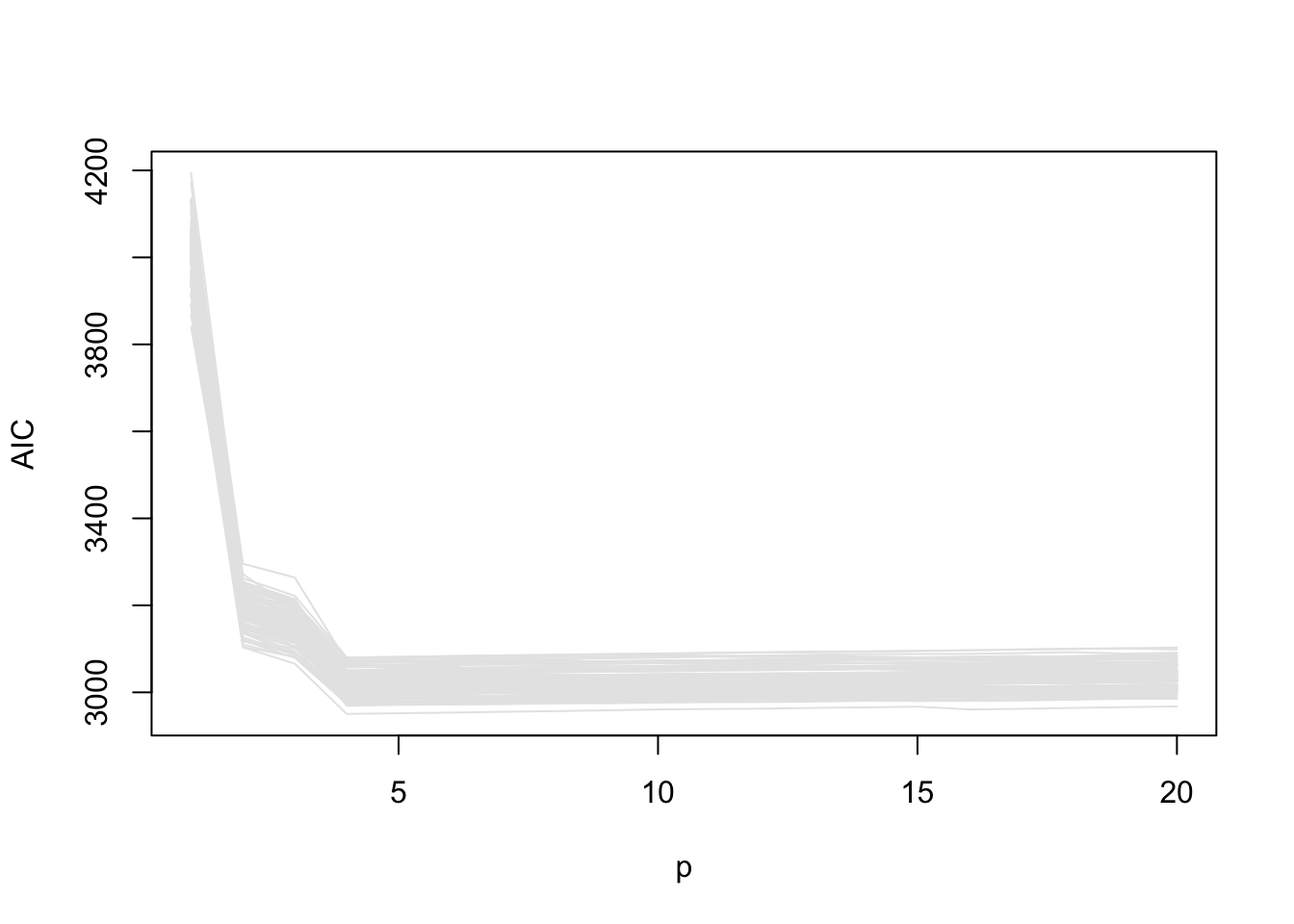
The code chunk below will run the required simulations and store the results in the list res_true.
set.seed(1)

ns <- c(25, 50, 100, 1000)
res_true <- as.list(numeric(length(ns)))
for (j in 1:length(ns)) {
    res_true[[j]] <- run_simulation(n = ns[j], M = 3, pmax = 20, B = 100,
                                    w = function(x) 0.001 * (100 + x + x^2 + x^3))
}
names(res_true) <- paste("n =", ns)
Let’s investigate the behaviour of AIC.
sapply(res_true, function(x) get_selection_counts(x$AIC))$`n = 25`
ic_order
4 5 6 7 8 9 10 18
67 11 11 2 5 1 1 2
$`n = 50`
ic_order
4 5 6 7 8 9 11 13
70 7 10 5 3 1 3 1
$`n = 100`
ic_order
4 5 6 7 8 9 18
72 11 8 5 2 1 1
$`n = 1000`
ic_order
4 5 6 7 8 9 10 11
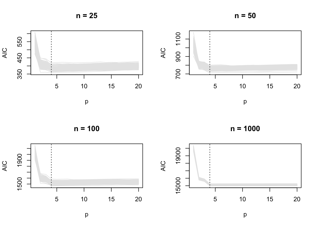
69 11 10 4 2 2 1 1 AIC behaves similarly for all \(n\). In all cases, the correct (cubic) model is preferred most of the time, but the probability of it being selected does not tend to one as \(n\) grows. This is also apparent in the the AIC vs \(p\) plots
par(mfrow = c(2, 2))
for (j in 1:length(ns)) {
    plot_ic(res_true[[j]]$AIC, ylab = "AIC", main = paste("n =", ns[j]))
    abline(v = 4, lty = 3)
}
Let’s explore the behaviour of BIC.
sapply(res_true, function(x) get_selection_counts(x$BIC))$`n = 25`
ic_order
2 3 4 5 6
1 1 93 4 1
$`n = 50`
ic_order
4 5
99 1
$`n = 100`
ic_order
4 5
97 3
$`n = 1000`
ic_order
4
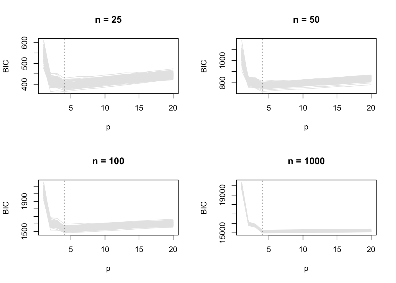
100 In this example, the set of candidate models includes the model we simulate from, and BIC selects the correct model more and more often as \(n\) increases. This is also apparent in the BIC vs \(p\) plots.
par(mfrow = c(2, 2))
for (j in 1:length(ns)) {
    plot_ic(res_true[[j]]$BIC, ylab = "BIC", main = paste("n =", ns[j]))
    abline(v = 4, lty = 3)
}
- The code chunk below will run the required simulations and store the results in the list
res_other.
set.seed(1)

ns <- c(25, 50, 100, 1000)
res_other <- as.list(numeric(length(ns)))
for (j in 1:length(ns)) {
    res_other[[j]] <- run_simulation(n = ns[j], M = 3, pmax = 20, B = 100,
                                     w = function(x) 1.2 / (1 + exp( - x)))
}
names(res_other) <- paste("n =", ns)
Let’s investigate the behaviour of AIC.
sapply(res_other, function(x) get_selection_counts(x$AIC))$`n = 25`
ic_order
4 5 6 7 8 9 10 11 12 13 14 15 16 20
9 2 33 8 19 5 7 3 4 2 2 4 1 1
$`n = 50`
ic_order
4 6 7 8 9 10 11 12 13 14 15 16 17 18 20
1 31 5 22 10 8 5 4 1 3 3 3 1 2 1
$`n = 100`
ic_order
6 7 8 9 10 11 12 13 16 17 18
15 3 33 10 28 2 3 1 1 2 2
$`n = 1000`
ic_order
10 11 12 13 14 15 16 17 18 20
13 5 33 6 21 5 8 1 7 1 As \(n\) increases, AIC tends to select increasingly complex models, which provide a better approximation to the true distribution which generated the data, which is not a polynomial model.
On the other hand, BIC prefers simpler models to AIC, although it still tends to prefer more complex models as \(n\) increases in this case.
sapply(res_other, function(x) get_selection_counts(x$BIC))$`n = 25`
ic_order
4 5 6 7 8 10 13
41 4 43 5 5 1 1
$`n = 50`
ic_order
4 5 6 7 8 9 10
18 2 59 9 10 1 1
$`n = 100`
ic_order
6 7 8 10
55 6 35 4
$`n = 1000`
ic_order
8 10 11 12 13
13 76 3 7 1 - We have shown that \[ \bar\ell(\hat\theta) - p / (n M) = -\frac{1}{2nM} \{2 (p - \ell(\hat\theta))\} = -\frac{1}{2nM} AIC \] is a bias-corrected estimator of \(\Delta\).
So, \[ \tilde{\Delta} = - \frac{1}{2nM} \mathop{\mathrm{E}}(AIC) \, , \] should be approaching \(\Delta\) as \(n\) increases. We can estimate \(\tilde{\Delta}\) empirically by transforming the AIC values we obtained in the simulations, and taking averages for every \(p\).
A direct, simulation-based estimator of \(\Delta\) can be obtained by its definition, using independent samples from the ones that are used for estimation. The code chunk below provides a function that returns a simulation-base estimator of \(\Delta\) as a function of \(p\).
estimate_Delta <- function(n, M = 3, pmax = 20, B = 100,
                           w =  function(x) 0.001 * (100 + x + x^2 + x^3)) {
    mu <- function(x) {
        8 * exp(w(x))
    }
    x <- rep(seq(from = -10, to = 10, length = n), each = M)
    ## Object to hold out-of-sample log-likelihood
    oo_ll <- matrix(NA, nrow = B, ncol = pmax)
    for (b in 1:B) {
        ## Simulate responses
        y <- rpois(n = M * n, lambda = mu(x))
        y_plus <- rpois(n = M * n, lambda = mu(x))
        ## Fit intercept-only model and compute out-of-sample log-likelihood
        mod <- glm(y ~ 1, family = poisson)
        oo_ll[b, 1] <- sum(dpois(y_plus, fitted(mod), log = TRUE))
        ## Fit remaining models and compute out-of-sample log-likelihood
        for(p in 2:pmax) {
            modp <- glm(y ~ poly(x, p - 1), family = poisson)
            oo_ll[b, p] <- sum(dpois(y_plus, fitted(modp), log = TRUE))
        }
    }
    colMeans(oo_ll / (n * M))
}
The estimates of \(\Delta\) for \(w(x) = 0.001 \left( 100 + x + x^2 + x^3 \right)\) and \(w(x) = 1.2/\{1 + \exp(-x)\}\) are
set.seed(1)
ns <- c(25, 50, 100, 1000)
Delta_true <- Delta_other <- as.list(numeric(length(ns)))
for (j in 1:length(ns)) {
Delta_true[[j]] <- estimate_Delta(n = ns[j], M = 3, pmax = 20, B = 100,
w = function(x) 0.001 * (100 + x + x^2 + x^3))
Delta_other[[j]] <- estimate_Delta(n = ns[j], M = 3, pmax = 20, B = 100,
w = function(x) 1.2 / (1 + exp( - x)))
}
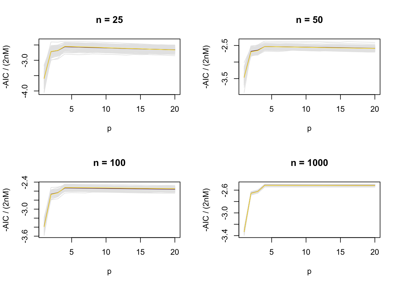
names(Delta_true) <- names(Delta_other) <- paste("n =", ns)For \(w(x) = 0.001 \left( 100 + x + x^2 + x^3 \right)\), we get
cols <- hcl.colors(2)
par(mfrow = c(2, 2))
for (j in 1:length(ns)) {
    Delta_t <- - res_true[[j]]$AIC / (2 * ns[j] * M)
    plot_ic(Delta_t, ylab = "-AIC / (2nM)", main = paste("n =", ns[j]))
    lines(1:pmax, colMeans(Delta_t), col = cols[1])
    lines(1:pmax, Delta_true[[j]], col = cols[2])
}
and for \(w(x) = 1.2/\{1 + \exp(-x)\}\), we get
par(mfrow = c(2, 2))
for (j in 1:length(ns)) {
    Delta_t <- - res_other[[j]]$AIC / (2 * ns[j] * M)
    plot_ic(Delta_t, ylab = "-AIC / (2nM)", main = paste("n =", ns[j]))
    lines(1:pmax, colMeans(Delta_t), col = cols[1])
    lines(1:pmax, Delta_other[[j]], col = cols[2])
}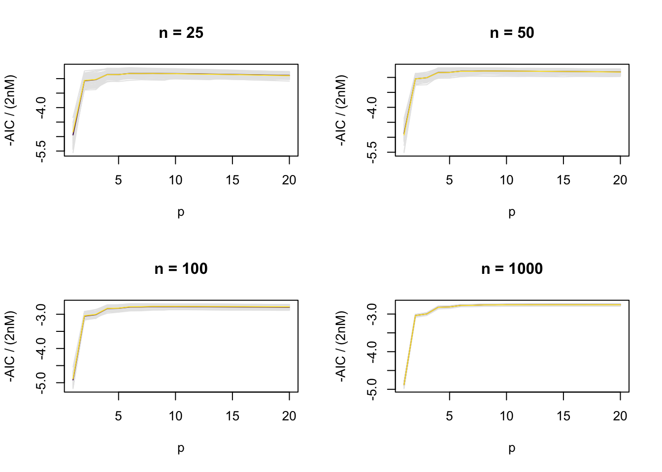
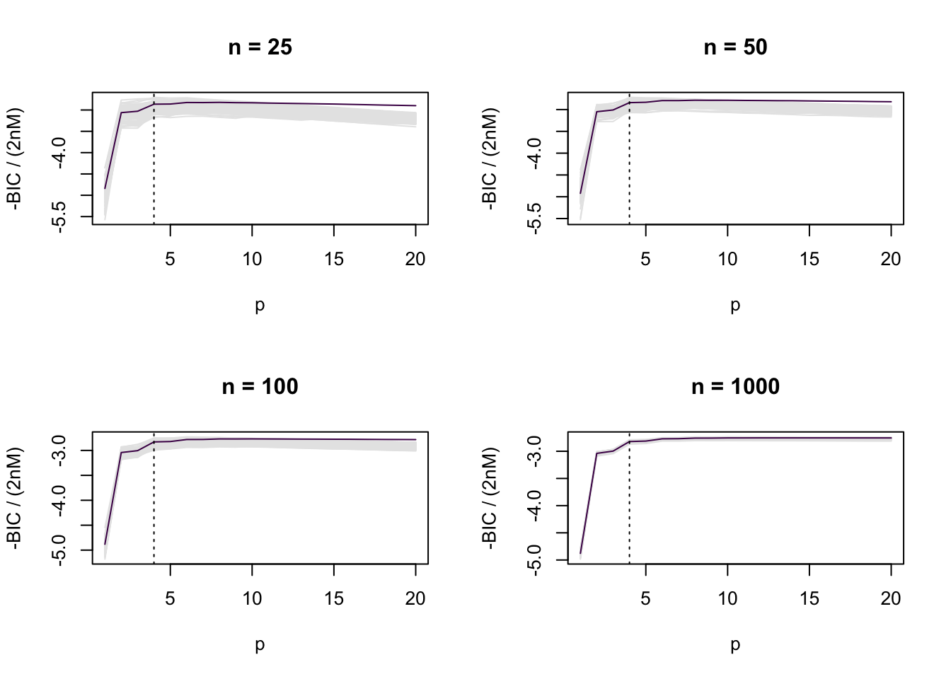
The purple piecewise linear functions are the simulation-based estimates of \(\Delta\) based on AIC, and the yellow piecewise linear functions are the simulation-based estimates of \(\Delta\) based on its definition. In the current setting, we can see that the two simulation-based estimates are almost identical in value.
The fact that BIC does not estimate \(\Delta\) can now be made directly apparent. For example, for \(w(x) = 1.2/\{1 + \exp(-x)\}\),
par(mfrow = c(2, 2))
for (j in 1:length(ns)) {
    plot_ic(- res_other[[j]]$BIC / (2 * ns[j] * M), ylab = "-BIC / (2nM)", main = paste("n =", ns[j]))
    lines(1:pmax, Delta_other[[j]], col = cols[1])
    abline(v = 4, lty = 3)
}